Learning Objectives
In this lab, you will play with unsupervised classification techniques while working with ecological community datasets.
Ordination orders sites near each other based on similarity. It is a multivariate analysis technique used to effectively collapse dependent axes into fewer dimensions, i.e. dimensionality reduction.
Principal Components Analyses (PCA) is the most common and oldest technique that assumes linear relationships between axes. You will follow a non-ecological example from Chapter 17 Principal Components Analysis | Hands-On Machine Learning with R to learn about this commonly used technique.
Non-metric MultiDimensional Scaling (NMDS) allows for non-linear relationships. This ordination technique is implemented in the R package
vegan. You’ll use an ecological dataset, species and environment from lichen pastures that reindeer forage upon, with excerpts from the vegantutor vignette (source) to apply these techniques:- Unconstrained ordination on species using NMDS;
- Overlay with environmental gradients; and
- Constrained ordination on species and environmnent using another ordination technique, canonical correspondence analysis (CCA).
1 Ordination
Ordination orders sites near each other based on similarity. It is a multivariate analysis technique used to effectively collapse dependent axes into fewer dimensions, i.e. “dimensionality reduction.” It also falls into the class of unsupervised learning because a “response term” is not used to fit the model.
1.1 Principal Components Analysis (PCA)
Although this example uses a non-ecological dataset, it walks through the idea and procedure of conducting an ordination using the most widespread technique of PCA.
Please read the entirety of Chapter 17 Principal Components Analysis | Hands-On Machine Learning with R. Supporting text is mentioned below where code is run.
1.1.1 Prerequisites
See supporting text: 17.1 Prerequisites
Load the libraries and data. Set the seed of the random number generator for reproducible results. Inspect the data structure of the example my_basket dataset.
# load R packages
librarian::shelf(
  dplyr, ggplot2, h2o)

# set seed for reproducible results
set.seed(42)

# get data
url <- "https://koalaverse.github.io/homlr/data/my_basket.csv"
my_basket <- readr::read_csv(url)
dim(my_basket)
[1] 2000 42my_basket
# A tibble: 2,000 × 42
   `7up` lasagna pepsi   yop red.wine cheese   bbq bulmers mayonnaise
   <dbl>   <dbl> <dbl> <dbl>    <dbl>  <dbl> <dbl>   <dbl>      <dbl>
 1     0       0     0     0        0      0     0       0          0
 2     0       0     0     0        0      0     0       0          0
 3     0       0     0     0        0      0     0       0          0
 4     0       0     0     2        1      0     0       0          0
 5     0       0     0     0        0      0     0       2          0
 6     0       0     0     0        0      0     0       0          0
 7     1       1     0     0        0      0     1       0          0
 8     0       0     0     0        0      0     0       0          0
 9     0       1     0     0        0      0     0       0          0
10     0       0     0     0        0      0     0       0          0
# … with 1,990 more rows, and 33 more variables: horlics <dbl>,
#   chicken.tikka <dbl>, milk <dbl>, mars <dbl>, coke <dbl>,
#   lottery <dbl>, bread <dbl>, pizza <dbl>, sunny.delight <dbl>,
#   ham <dbl>, lettuce <dbl>, kronenbourg <dbl>, leeks <dbl>,
#   fanta <dbl>, tea <dbl>, whiskey <dbl>, peas <dbl>,
#   newspaper <dbl>, muesli <dbl>, white.wine <dbl>, carrots <dbl>,
#   spinach <dbl>, pate <dbl>, instant.coffee <dbl>, twix <dbl>, …
So each row is a grocery trip and each column a different grocery item. The cell represents the count of that grocery item for that trip. This is analogous to each row being a site and each column being a count of species. Here are more details on the dataset from Section 1.4:
my_basket.csv: Grocery items and quantities purchased. Each observation represents a single basket of goods that were purchased together.- Problem type: unsupervised basket analysis
- response variable: NA
- features: 42
- observations: 2,000
- objective: use attributes of each basket to identify common groupings of items purchased together.
1.1.2 Performing PCA in R
What does “reducing the dimensionality” really mean? Let’s look at the “dimensions” of this my_basket dataset with the dim() function.
dim(my_basket)
[1] 2000 42So the dimensions are 2000 rows (i.e. grocery trips) by 42 columns (i.e. grocery items).
A single ordination component “reduces the dimensionality” of the dataset by collapsing all the columns (e.g., grocery items or species) into a single column of values ordering all rows (e.g., grocery trips or sites) based on similarity. This component can be plotted as row labels along a straight line (like the x axis alone). This component is derived from applying “weightings” to each item as an eigenvector and can only explain a proportion of the variance contained across all columns. So each ordination axes is composed of different weightings, or influence, across the input columns. Adding ordination components, i.e. additional summarizing columns, explains more variance but expands the “dimensionality” (i.e. columns). So a second component could also be plotted as row labels along a straight line and combined in a plot with the first component to produce a row label for the intersection of x as the first component PC1 and y as the second component. A 3D plot with a z axis could render a third component PC3. Additional components can be added up to the number of input columns for explaining all the variation, but we’re limited to 3 axes for visualization so we can mix and match which ordination to plot on which axes.
See supporting text: 17.4 Performing PCA in R
h2o.no_progress()  # turn off progress bars for brevity
h2o.init(max_mem_size = "5g")  # connect to H2O instance
 Connection successful!

R is connected to the H2O cluster:
    H2O cluster uptime:         8 days 4 hours
    H2O cluster timezone:       America/Los_Angeles
    H2O data parsing timezone:  UTC
    H2O cluster version:        3.36.0.1
    H2O cluster version age:    1 month and 9 days
    H2O cluster name:           H2O_started_from_R_bbest_qea893
    H2O cluster total nodes:    1
    H2O cluster total memory:   4.99 GB
    H2O cluster total cores:    12
    H2O cluster allowed cores:  12
    H2O cluster healthy:        TRUE
    H2O Connection ip:          localhost
    H2O Connection port:        54321
    H2O Connection proxy:       NA
    H2O Internal Security:      FALSE
    H2O API Extensions:         Amazon S3, XGBoost, Algos, Infogram, AutoML, Core V3, TargetEncoder, Core V4
    R Version:                  R version 4.1.1 (2021-08-10)
# convert data to h2o object
my_basket.h2o <- as.h2o(my_basket)
# run PCA
my_pca <- h2o.prcomp(
training_frame = my_basket.h2o,
pca_method = "GramSVD",
k = ncol(my_basket.h2o),
transform = "STANDARDIZE",
impute_missing = TRUE,
max_runtime_secs = 1000)
my_pca
Model Details:
==============
H2ODimReductionModel: pca
Model ID: PCA_model_R_1643572539291_26
Importance of components:
pc1 pc2 pc3 pc4 pc5
Standard deviation 1.513919 1.473768 1.459114 1.440635 1.435279
Proportion of Variance 0.054570 0.051714 0.050691 0.049415 0.049048
Cumulative Proportion 0.054570 0.106284 0.156975 0.206390 0.255438
pc6 pc7 pc8 pc9 pc10
Standard deviation 1.411544 1.253307 1.026387 1.010238 1.007253
Proportion of Variance 0.047439 0.037400 0.025083 0.024300 0.024156
Cumulative Proportion 0.302878 0.340277 0.365360 0.389659 0.413816
pc11 pc12 pc13 pc14 pc15
Standard deviation 0.988724 0.985320 0.970453 0.964303 0.951610
Proportion of Variance 0.023276 0.023116 0.022423 0.022140 0.021561
Cumulative Proportion 0.437091 0.460207 0.482630 0.504770 0.526331
pc16 pc17 pc18 pc19 pc20
Standard deviation 0.947978 0.944826 0.932943 0.931745 0.924207
Proportion of Variance 0.021397 0.021255 0.020723 0.020670 0.020337
Cumulative Proportion 0.547728 0.568982 0.589706 0.610376 0.630713
pc21 pc22 pc23 pc24 pc25
Standard deviation 0.917106 0.908494 0.903247 0.898109 0.894277
Proportion of Variance 0.020026 0.019651 0.019425 0.019205 0.019041
Cumulative Proportion 0.650739 0.670390 0.689815 0.709020 0.728061
pc26 pc27 pc28 pc29 pc30
Standard deviation 0.876167 0.871809 0.865912 0.855036 0.845130
Proportion of Variance 0.018278 0.018096 0.017852 0.017407 0.017006
Cumulative Proportion 0.746339 0.764436 0.782288 0.799695 0.816701
pc31 pc32 pc33 pc34 pc35
Standard deviation 0.842818 0.837655 0.826422 0.818532 0.813796
Proportion of Variance 0.016913 0.016706 0.016261 0.015952 0.015768
Cumulative Proportion 0.833614 0.850320 0.866581 0.882534 0.898302
pc36 pc37 pc38 pc39 pc40
Standard deviation 0.804380 0.796073 0.793781 0.780615 0.778612
Proportion of Variance 0.015405 0.015089 0.015002 0.014509 0.014434
Cumulative Proportion 0.913707 0.928796 0.943798 0.958307 0.972741
pc41 pc42
Standard deviation 0.763433 0.749696
Proportion of Variance 0.013877 0.013382
Cumulative Proportion 0.986618 1.000000
H2ODimReductionMetrics: pca
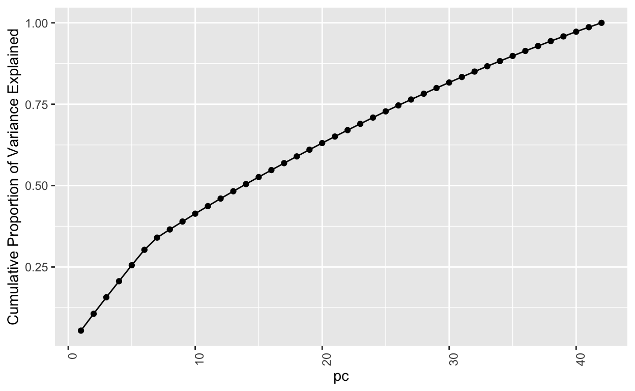
No model metrics available for PCASo the number of ordinations is set to the number of columns initially. That means that all 42 ordinations can explain all the variability, i.e. 100% or 1. Let’s add a plot to show this explicitly based on information above cumulatively adding the Proportion of Variance from each subsequent principal component pc.
my_pca@model$model_summary %>%
  add_rownames() %>%
  tidyr::pivot_longer(-rowname) %>%
  filter(
    rowname == "Proportion of Variance") %>%
  mutate(
    pc = stringr::str_replace(name, "pc", "") %>% as.integer()) %>%
  ggplot(aes(x = pc, y=cumsum(value))) +
  geom_point() + geom_line() +
  theme(axis.text.x = element_text(angle=90, hjust = 1))  +
  ylab("Cumulative Proportion of Variance Explained")
Next, let’s take a closer look at a single principal component pc1. It has these “weightings” associated with each of the input columns.
my_pca@model$eigenvectors %>%
  as.data.frame() %>%
  mutate(feature = row.names(.)) %>%
  ggplot(aes(pc1, reorder(feature, pc1))) +
  geom_point()
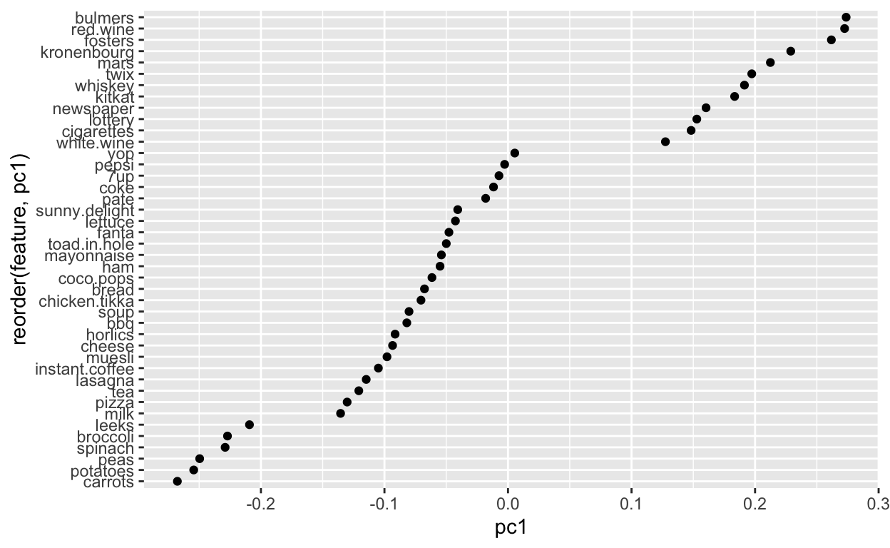
So positive values are associated with more ‘hedonistic/impulse’ items like beer, wine, chocolate, lottery and cigarettes. Whereas ‘healthy’ items align along the negative like carrots, peas, spinach and broccoli. That makes sense that these items are more likely to be clustered on a given shopping trip.
Now let’s look at two ordination components at once by plotting pc1 on the x axis and pc2 on the y axis.
my_pca@model$eigenvectors %>%
  as.data.frame() %>%
  mutate(feature = row.names(.)) %>%
  ggplot(aes(pc1, pc2, label = feature)) +
  geom_text()
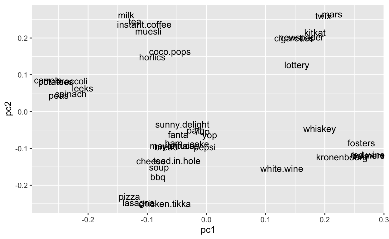
So clusters of proximate items are more likely to co-occur on a given grocery trip. Again, this is analagous to species more likely to co-occur at a given site. And the spread of the species is based on the weightings along each axes.
1.1.3 Eigenvalue criterion
See supporting text: 17.5.1 Eigenvalue criterion.
# Compute eigenvalues
eigen <- my_pca@model$importance["Standard deviation", ] %>%
  as.vector() %>%
  .^2

# Sum of all eigenvalues equals number of variables
sum(eigen)
[1] 42## [1] 42
# Find PCs where the sum of eigenvalues is greater than or equal to 1
which(eigen >= 1)
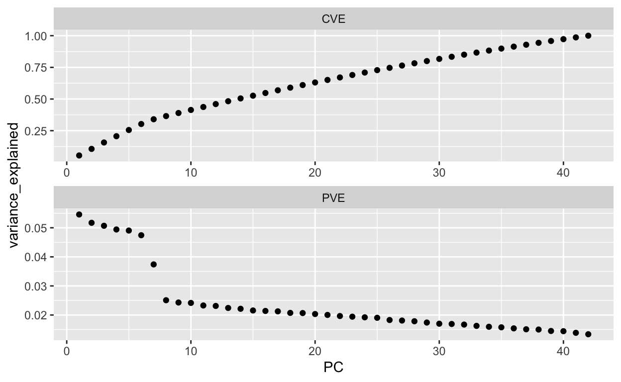
[1] 1 2 3 4 5 6 7 8 9 10# Extract PVE and CVE
ve <- data.frame(
PC = my_pca@model$importance %>% seq_along(),
PVE = my_pca@model$importance %>% .[2,] %>% unlist(),
CVE = my_pca@model$importance %>% .[3,] %>% unlist())
# Plot PVE and CVE
ve %>%
tidyr::gather(metric, variance_explained, -PC) %>%
ggplot(aes(PC, variance_explained)) +
geom_point() +
facet_wrap(~ metric, ncol = 1, scales = "free")
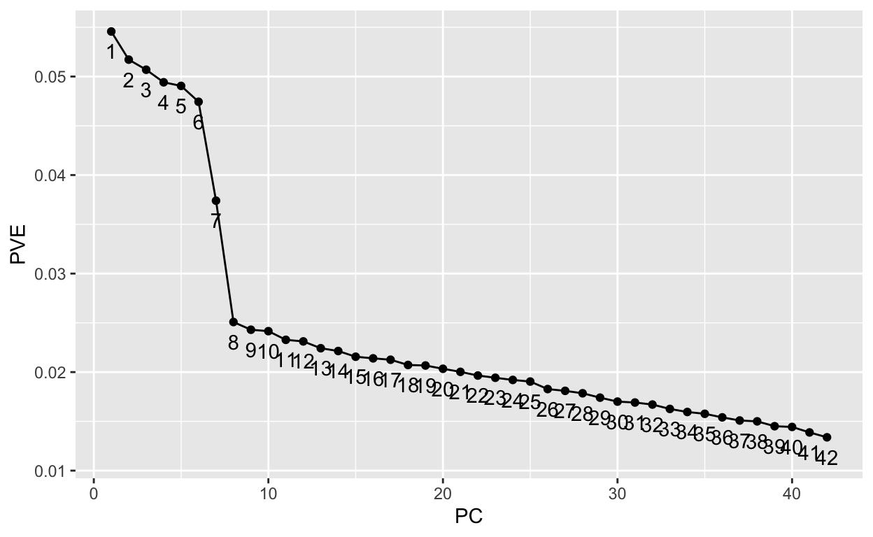
[1] 27# Screee plot criterion
data.frame(
PC = my_pca@model$importance %>% seq_along,
PVE = my_pca@model$importance %>% .[2,] %>% unlist()) %>%
ggplot(aes(PC, PVE, group = 1, label = PC)) +
geom_point() +
geom_line() +
geom_text(nudge_y = -.002)
1.2 Non-metric MultiDimensional Scaling (NMDS)
Non-metric MultiDimensional Scaling (NMDS) is probably the most common ordination technique in ecology. It can account for non-linear relationships unlike PCA, but requires some ensemble averaging to account for differing results from different initial conditions, which accounts for the preference for metaMDS() to get at the average of many model fits versus a single NMDS solution from monoMDS().
1.2.1 Unconstrained Ordination on Species
See supporting text: 2.1 Non-metric Multidimensional scaling in vegantutor.pdf.
“Unconstrained ordination” refers to ordination of sites by species, “unconstrained” by the environment. Biodiversity within a site is also called alpha \(\alpha\) diversity and biodiversity across sites is called beta \(\beta\) diversity.
The varespecies dataset describes the cover of species (44 columns) across sites (24 rows) and varechem the soil chemistry (14 columns) across the same sites (24 rows).
# load R packages
librarian::shelf(
  vegan, vegan3d)

# vegetation and environment in lichen pastures from Vare et al (1995)
data("varespec") # species
data("varechem") # chemistry

if (interactive()){
  help(varechem)
  help(varespec)
}

varespec %>% tibble()
# A tibble: 24 × 44
Callvulg Empenigr Rhodtome Vaccmyrt Vaccviti Pinusylv Descflex
<dbl> <dbl> <dbl> <dbl> <dbl> <dbl> <dbl>
1 0.55 11.1 0 0 17.8 0.07 0
2 0.67 0.17 0 0.35 12.1 0.12 0
3 0.1 1.55 0 0 13.5 0.25 0
4 0 15.1 2.42 5.92 16.0 0 3.7
5 0 12.7 0 0 23.7 0.03 0
6 0 8.92 0 2.42 10.3 0.12 0.02
7 4.73 5.12 1.55 6.05 12.4 0.1 0.78
8 4.47 7.33 0 2.15 4.33 0.1 0
9 0 1.63 0.35 18.3 7.13 0.05 0.4
10 24.1 1.9 0.07 0.22 5.3 0.12 0
# … with 14 more rows, and 37 more variables: Betupube <dbl>,
# Vacculig <dbl>, Diphcomp <dbl>, Dicrsp <dbl>, Dicrfusc <dbl>,
# Dicrpoly <dbl>, Hylosple <dbl>, Pleuschr <dbl>, Polypili <dbl>,
# Polyjuni <dbl>, Polycomm <dbl>, Pohlnuta <dbl>, Ptilcili <dbl>,
# Barbhatc <dbl>, Cladarbu <dbl>, Cladrang <dbl>, Cladstel <dbl>,
# Cladunci <dbl>, Cladcocc <dbl>, Cladcorn <dbl>, Cladgrac <dbl>,
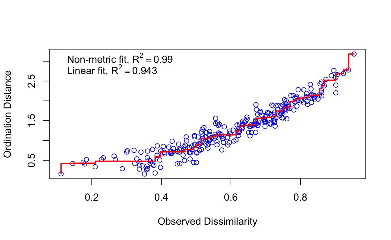
# Cladfimb <dbl>, Cladcris <dbl>, Cladchlo <dbl>, Cladbotr <dbl>, …The ordination is based on the ecological distance between sites (as rows) given the compositional similarity of the species (as columns). The PCA technique previously used created this distance matrix under the hood. Here we explicitly create it with vegdist() using the default Bray-Curtis method (see method="bray" in ?vegdist) discussed in the previous 2a Clustering lab. With monoMDS a single NMDS result using the default number of dimensions (see k=2 in ?monoMDS), and given the randomized nature of the algorithm your results may vary. The subsequent stressplot describes how well the ordination fits the observed dissimilarity. Each blue circle represents the ecological distance between two sites from the original data (“observed” x axis) compared to the fitted data (“ordination” y axis) as explained by the 2 dimensions (from using default k=2).
vare.dis <- vegdist(varespec)
vare.mds0 <- monoMDS(vare.dis)
stressplot(vare.mds0)
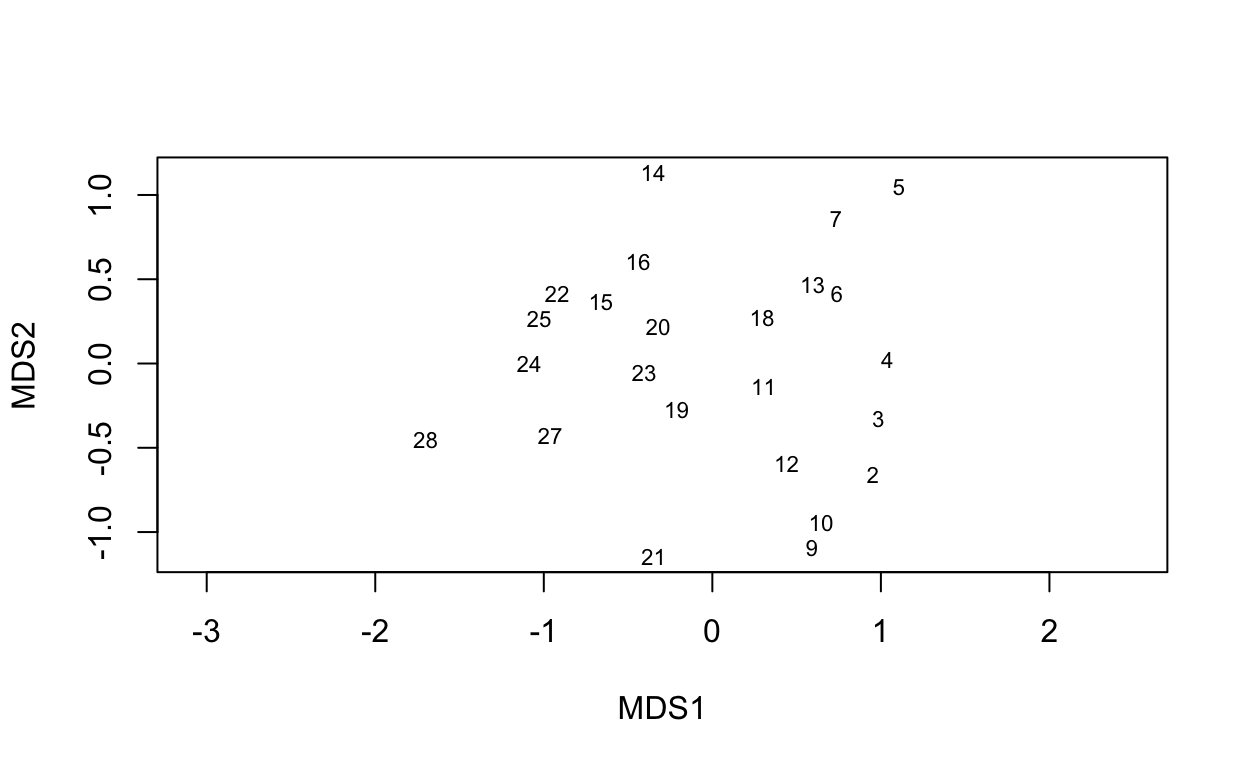
The ordiplot() shows the sites as ordered along the two dimensions. The option type = "t" is to show the text labels of those sites.
ordiplot(vare.mds0, type = "t")
Next, let’s use the full blown NMDS with extra model averaging (see ?metaMDS).
vare.mds <- metaMDS(varespec, trace = FALSE)
vare.mds
Call:
metaMDS(comm = varespec, trace = FALSE)

global Multidimensional Scaling using monoMDS

Data:     wisconsin(sqrt(varespec))
Distance: bray

Dimensions: 2
Stress:     0.1825658
Stress type 1, weak ties
No convergent solutions - best solution after 20 tries
Scaling: centring, PC rotation, halfchange scaling
Species: expanded scores based on 'wisconsin(sqrt(varespec))'
The “stress” is a measure of how well the ordination explains variation across the columns. A stress value around or above 0.2 is deemed suspect and a stress value approaching 0.3 indicates that the ordination is arbitrary. Stress values equal to or below 0.1 are considered fair, while values equal to or below 0.05 indicate good fit.
plot(vare.mds, type = "t")
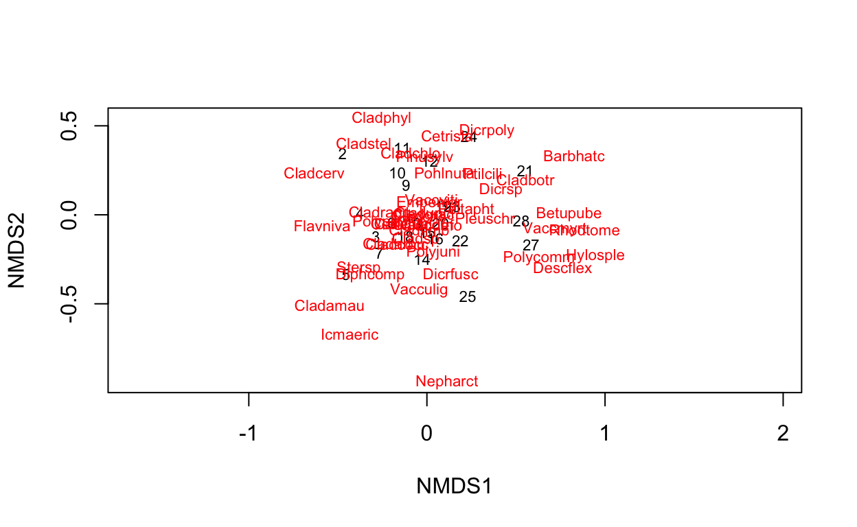
Now we’ve added the species in red to the plot indicating which sites are more likely to contain the labeled species.
1.2.2 Overlay with Environment
The following techniques do NOT change the ordination of the sites (that’s “constrained ordination”). Rather they visually describe the gradient of the environment given their position on the ordination axes.
See supporting text in vegantutor.pdf:
- 3 Environmental interpretation
- 3.1 Vector fitting
- 3.2 Surface fitting
ef <- envfit(vare.mds, varechem, permu = 999)
ef
***VECTORS

            NMDS1    NMDS2     r2 Pr(>r)
N        -0.05738 -0.99835 0.2536  0.046 *
P         0.61977  0.78478 0.1939  0.109
K         0.76653  0.64220 0.1809  0.121
Ca        0.68527  0.72829 0.4119  0.004 **
Mg        0.63258  0.77449 0.4270  0.004 **
S         0.19145  0.98150 0.1752  0.135
Al       -0.87156  0.49029 0.5269  0.001 ***
Fe       -0.93594  0.35215 0.4450  0.001 ***
Mn        0.79873 -0.60169 0.5231  0.002 **
Zn        0.61757  0.78652 0.1879  0.123
Mo       -0.90314  0.42935 0.0610  0.494
Baresoil  0.92479 -0.38047 0.2508  0.045 *
Humdepth  0.93279 -0.36042 0.5201  0.001 ***
pH       -0.64795  0.76168 0.2308  0.058 .
---
Signif. codes:  0 '***' 0.001 '**' 0.01 '*' 0.05 '.' 0.1 ' ' 1
Permutation: free
Number of permutations: 999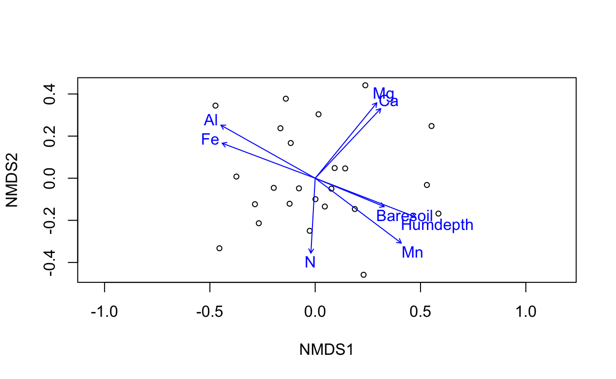
ef <- envfit(vare.mds ~ Al + Ca, data = varechem)
plot(vare.mds, display = "sites")
plot(ef)
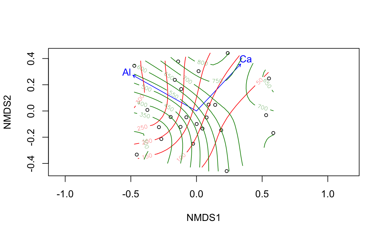
tmp <- with(varechem, ordisurf(vare.mds, Al, add = TRUE))
ordisurf(vare.mds ~ Ca, data=varechem, add = TRUE, col = "green4")
Family: gaussian
Link function: identity

Formula:
y ~ s(x1, x2, k = 10, bs = "tp", fx = FALSE)

Estimated degrees of freedom:
4.72  total = 5.72

REML score: 156.656
The ordination surface plot from ordisurf() displays contours of an environmental gradient across sites. It is a more detailed look at an environmental gradient compared to the single blue line vector. This environmental overlay is generated by fitting a GAM where the response is the environmental variable of interest and the predictors are a bivariate smooth of the ordination axes, all given by the formula: Ca ~ s(NMDS1, NMDS2) (Remember each site is associated with a position on the NMDS axes and has an environmental value). We can see from the code that the green4 color contours are for Calcium Ca.
1.2.3 Constrained Ordination on Species and Environment
See supporting text in vegantutor.pdf:
- 4 Constrained ordination
- 4.1 Model specification
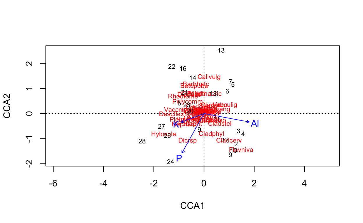
Technically, this uses another technique cca, or canonical correspondence analysis.
# ordinate on species constrained by three soil elements
vare.cca <- cca(varespec ~ Al + P + K, varechem)
vare.cca
Call: cca(formula = varespec ~ Al + P + K, data = varechem)

              Inertia Proportion Rank
Total          2.0832     1.0000
Constrained    0.6441     0.3092    3
Unconstrained  1.4391     0.6908   20
Inertia is scaled Chi-square

Eigenvalues for constrained axes:
  CCA1   CCA2   CCA3
0.3616 0.1700 0.1126

Eigenvalues for unconstrained axes:
   CA1    CA2    CA3    CA4    CA5    CA6    CA7    CA8
0.3500 0.2201 0.1851 0.1551 0.1351 0.1003 0.0773 0.0537
(Showing 8 of 20 unconstrained eigenvalues)
# plot ordination
plot(vare.cca)
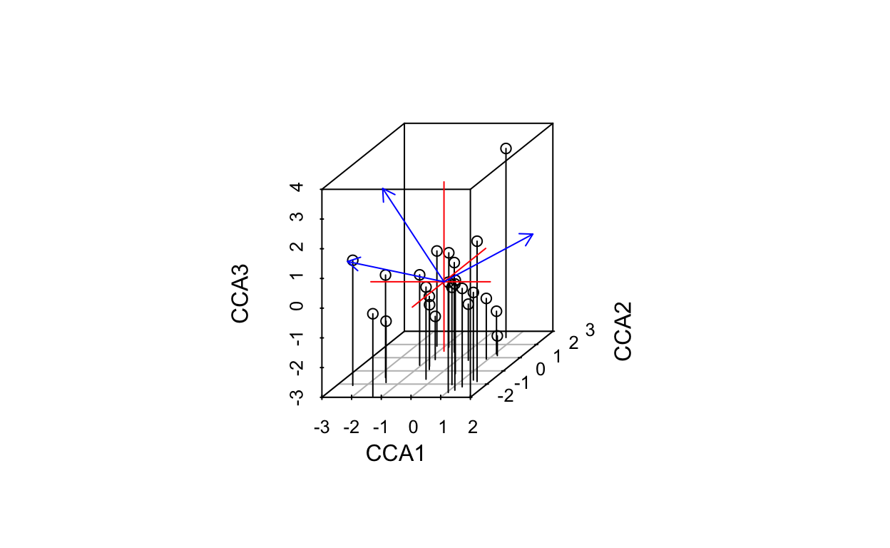
# plot 3 dimensions
ordiplot3d(vare.cca, type = "h")
if (interactive()){
  ordirgl(vare.cca)
}
2 Lab2 Submission
To submit Lab 2, please submit the path on taylor.bren.ucsb.edu to your single consolidated Rmarkdown document (i.e. combined from separate parts) that you successfully knitted here:
The path should start /Users/ and end in .Rmd. Please be sure to have succesfully knitted to html, as in I should see the .html file there by the same name with all the outputs.
In your lab, please be sure to include the following outputs and responses to questions: