Learning Objectives
- Explore
- Fetch species observations from the Global Biodiversity Information Facility (GBIF.org) using an R package that wraps a function around their API.
- Fetch environmental data for defining environmental relationship in the species distribution model (SDM).
- Generate pseudo-absences, or background, points with which to differentiate from the species presence points in the SDM.
- Extract underlying environmental data from points.
- Plot term plots of each environmental predictor with the species response.
1 Overview
This lab will introduce you to machine learning by predicting presence of a species of you choosing from observations and environmental data. We will largely follow guidance found at Species distribution modeling | R Spatial using slightly newer R packages and functions.
2 Explore
This first part of the lab involves fetching data for your species of interest, whether terrestrial or marine.
2.1 Install Packages
You’ll need to have the following R Software installed:
You’re also encouraged to use git to version your code, ideally in a Github repository.
You’ll use the librarian::shelf() function to load required software packages, installing them if needed.
# load packages, installing if missing
if (!require(librarian)){
  install.packages("librarian")
  library(librarian)
}
librarian::shelf(
  dismo, dplyr, DT, ggplot2, here, htmltools, leaflet, mapview, purrr, raster, readr, rgbif, rgdal, rJava, sdmpredictors, sf, spocc, tidyr)
select <- dplyr::select # overwrite raster::select
options(readr.show_col_types = FALSE)

# set random seed for reproducibility
set.seed(42)

# directory to store data
dir_data <- here("data/sdm")
dir.create(dir_data, showWarnings = F, recursive = T)
If you have a problem installing the rJava package like so:

Please install the Java Virtual Machine (JVM) for your operating system by visiting these links:
- rJava - Troubleshooting
- Oracle Java Dev Kit Download
- rJava fails to load · Issue #2254 · rstudio/rstudio
- If on MacOS or Linux, be sure to run
sudo R CMD javareconffrom the Terminal, then restart your computer and try in the R Consolelibrarian::shelf(rJava).
If you’re on a new Mac with the M1 processor, you might need to install the latest ARM 64-bit dmg for macOS from Azul Downloads (e.g. zulu17.30.15-ca-jdk17.0.1-macosx_aarch64.dmg).
2.2 Choose a Species
Please enter your species of choice for this lab here:
- Lab 1. Choose Species Google Form
Be sure to check nobody already chose this species here:
- Lab 1. Choose Species (Responses) Google Sheet
I also highly recommend choosing a species with at least 100 occurrences (try code below first). You can edit your choice through the form.
2.3 Get Species Observations
For illustrative purposes, I’ll choose the Brown-throated sloth (Bradypus variegatus) since we’re going to start slow with Machine Learning.

obs_csv <- file.path(dir_data, "obs.csv")
obs_geo <- file.path(dir_data, "obs.geojson")
redo    <- FALSE

if (!file.exists(obs_geo) | redo){
  # get species occurrence data from GBIF with coordinates
  (res <- spocc::occ(
    query = 'Bradypus variegatus',
    from = 'gbif', has_coords = T))

  # extract data frame from result
  df <- res$gbif$data[[1]]
  readr::write_csv(df, obs_csv)

  # convert to points of observation from lon/lat columns in data frame
  obs <- df %>%
    sf::st_as_sf(
      coords = c("longitude", "latitude"),
      crs = st_crs(4326)) %>%
    select(prov, key) # save space (joinable from obs_csv)
  sf::write_sf(obs, obs_geo, delete_dsn=T)
}
obs <- sf::read_sf(obs_geo)
nrow(obs) # number of rows
[1] 500# show points on map
mapview::mapview(obs, map.types = "Stamen.Terrain")
Code Tweak 1. Swap your own species name, ie not
"Bradypus variegatus".Code Tweak 2. Update your
occ()function to return a maximum of 10,000 records. (Hint:?occ)Code Tweak 3. Swap out the base map with a different basemap provider other than
Stamen.Terrain. View various options for leaflet-providers.Question 1. How many observations total are in GBIF for your species? (Hint:
?occ)Question 2. Do you see any odd observations, like marine species on land or vice versa? If so, please see the Data Cleaning and explain what you did to fix or remove these points.
2.4 Get Environmental Data
Next, you’ll use the Species Distribution Model predictors R package sdmpredictors to get underlying environmental data for your observations. First you’ll get underlying environmental data for predicting the niche on the species observations. Then you’ll generate pseudo-absence points with which to sample the environment. The model will differentiate the environment of the presence points from the pseudo-absence points.
2.4.1 Presence
dir_env <- file.path(dir_data, "env")

# set a default data directory
options(sdmpredictors_datadir = dir_env)

# choosing terrestrial
env_datasets <- sdmpredictors::list_datasets(terrestrial = TRUE, marine = FALSE)

# show table of datasets
env_datasets %>%
  select(dataset_code, description, citation) %>%
  DT::datatable()
# choose datasets for a vector
env_datasets_vec <- c("WorldClim", "ENVIREM")

# get layers
env_layers <- sdmpredictors::list_layers(env_datasets_vec)
DT::datatable(env_layers)
# choose layers after some inspection and perhaps consulting literature
env_layers_vec <- c("WC_alt", "WC_bio1", "WC_bio2", "ER_tri", "ER_topoWet")

# get layers
env_stack <- load_layers(env_layers_vec)

# interactive plot layers, hiding all but first (select others)
# mapview(env_stack, hide = T) # makes the html too big for Github
plot(env_stack, nc=2)
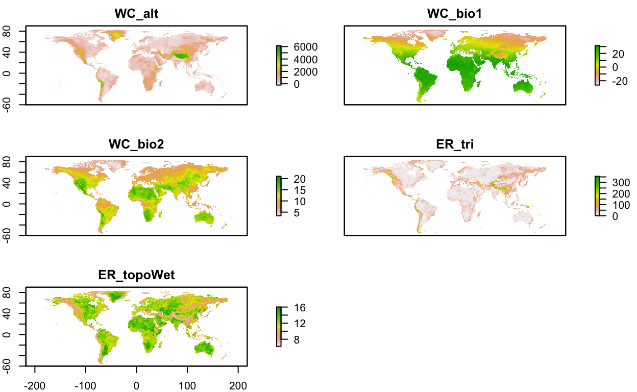
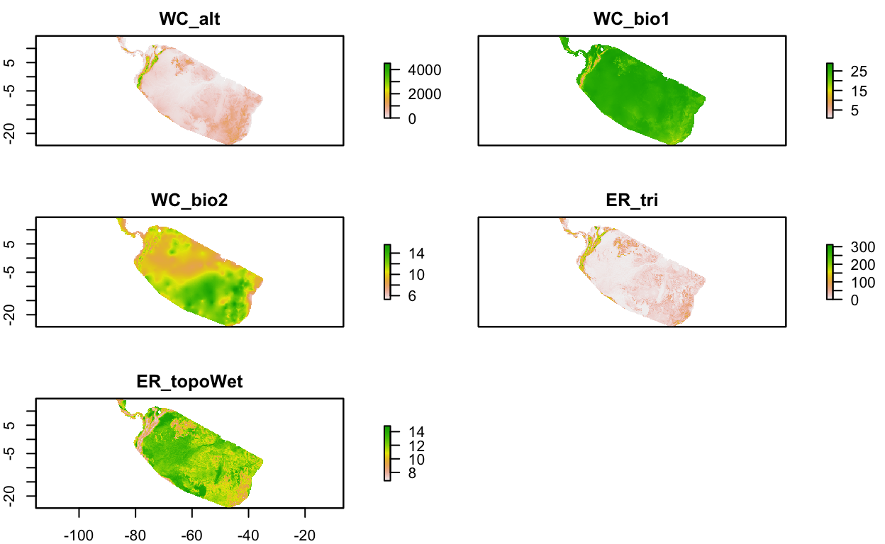
Notice how the extent is currently global for the layers. Let’s crop the environmental rasters to a reasonable study area around our species observations.
obs_hull_geo  <- file.path(dir_data, "obs_hull.geojson")
env_stack_grd <- file.path(dir_data, "env_stack.grd")

if (!file.exists(obs_hull_geo) | redo){
  # make convex hull around points of observation
  obs_hull <- sf::st_convex_hull(st_union(obs))

  # save obs hull
  write_sf(obs_hull, obs_hull_geo)
}
obs_hull <- read_sf(obs_hull_geo)

# show points on map
mapview(
  list(obs, obs_hull))
if (!file.exists(env_stack_grd) | redo){
  obs_hull_sp <- sf::as_Spatial(obs_hull)
  env_stack <- raster::mask(env_stack, obs_hull_sp) %>%
    raster::crop(extent(obs_hull_sp))
  writeRaster(env_stack, env_stack_grd, overwrite=T)
}
env_stack <- stack(env_stack_grd)

# show map
# mapview(obs) +
#   mapview(env_stack, hide = T) # makes html too big for Github
plot(env_stack, nc=2)
2.4.2 Pseudo-Absence
absence_geo <- file.path(dir_data, "absence.geojson")
pts_geo     <- file.path(dir_data, "pts.geojson")
pts_env_csv <- file.path(dir_data, "pts_env.csv")

if (!file.exists(absence_geo) | redo){
  # get raster count of observations
  r_obs <- rasterize(
    sf::as_Spatial(obs), env_stack[[1]], field=1, fun='count')

  # show map
  # mapview(obs) +
  #   mapview(r_obs)

  # create mask for
  r_mask <- mask(env_stack[[1]] > -Inf, r_obs, inverse=T)

  # generate random points inside mask
  absence <- dismo::randomPoints(r_mask, nrow(obs)) %>%
    as_tibble() %>%
    st_as_sf(coords = c("x", "y"), crs = 4326)

  write_sf(absence, absence_geo, delete_dsn=T)
}
absence <- read_sf(absence_geo)

# show map of presence, ie obs, and absence
mapview(obs, col.regions = "green") +
  mapview(absence, col.regions = "gray")
if (!file.exists(pts_env_csv) | redo){

  # combine presence and absence into single set of labeled points
  pts <- rbind(
    obs %>%
      mutate(
        present = 1) %>%
      select(present, key),
    absence %>%
      mutate(
        present = 0,
        key     = NA)) %>%
    mutate(
      ID = 1:n()) %>%
    relocate(ID)
  write_sf(pts, pts_geo, delete_dsn=T)

  # extract raster values for points
  pts_env <- raster::extract(env_stack, as_Spatial(pts), df=TRUE) %>%
    tibble() %>%
    # join present and geometry columns to raster value results for points
    left_join(
      pts %>%
        select(ID, present),
      by = "ID") %>%
    relocate(present, .after = ID) %>%
    # extract lon, lat as single columns
    mutate(
      #present = factor(present),
      lon = st_coordinates(geometry)[,1],
      lat = st_coordinates(geometry)[,2]) %>%
    select(-geometry)
  write_csv(pts_env, pts_env_csv)
}
pts_env <- read_csv(pts_env_csv)

pts_env %>%
  # show first 10 presence, last 10 absence
  slice(c(1:10, (nrow(pts_env)-9):nrow(pts_env))) %>%
  DT::datatable(
    rownames = F,
    options = list(
      dom = "t",
      pageLength = 20))
In the end this table is the data that feeds into our species distribution model (y ~ X), where:
yis thepresentcolumn with values of1(present) or0(absent)Xis all other columns: WC_alt, WC_bio1, WC_bio2, ER_tri, ER_topoWet, lon, lat
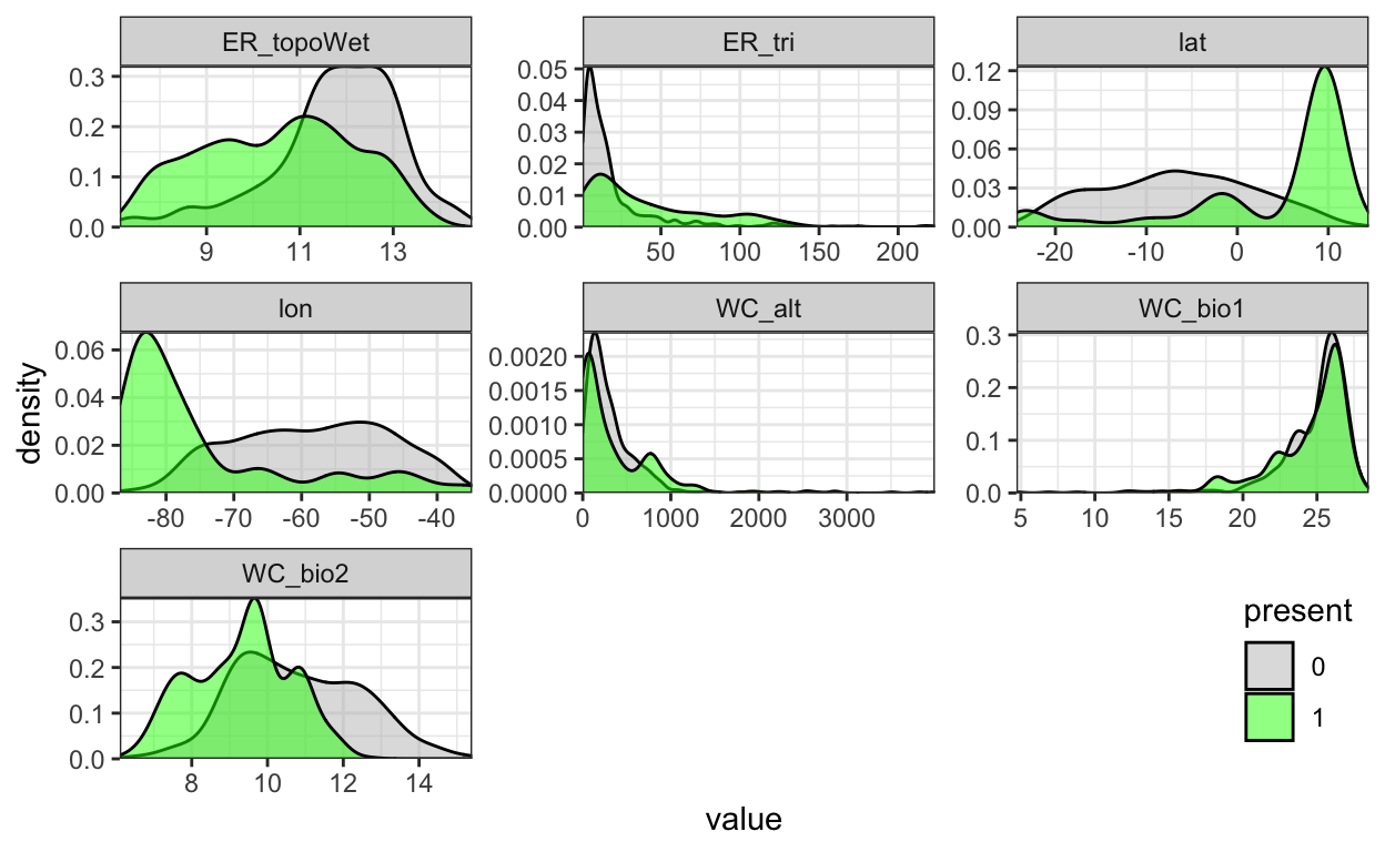
2.5 Term Plots
In the vein of exploratory data analyses, before going into modeling let’s look at the data. Specifically, let’s look at how obviously differentiated is the presence versus absence for each predictor – a more pronounced presence peak should make for a more confident model. A plot for a specific predictor and response is called a “term plot”. In this case we’ll look for predictors where the presence (present = 1) occupies a distinct “niche” from the background absence points (present = 0).
pts_env %>%
  select(-ID) %>%
  mutate(
    present = factor(present)) %>%
  pivot_longer(-present) %>%
  ggplot() +
  geom_density(aes(x = value, fill = present)) +
  scale_fill_manual(values = alpha(c("gray", "green"), 0.5)) +
  scale_x_continuous(expand=c(0,0)) +
  scale_y_continuous(expand=c(0,0)) +
  theme_bw() +
  facet_wrap(~name, scales = "free") +
  theme(
    legend.position = c(1, 0),
    legend.justification = c(1, 0))