Learning Objectives

There are two broad categories of Supervised Classification based on the type of response your modeling $y \sim x$, where $y$ is either a continuous value, in which case Regression, or it is a categorical value, in which case it’s a Classification.

A binary response, such as presence or absence, is a categorical value, so typically a Classification technique would be used. However, by transforming the response with a logit function, we were able to use Regression techniques like generalized linear (glm()) and generalized additive (gam()) models.

In this portion of the lab you’ll use Decision Trees as a Classification technique to the data with the response being categorical (factor(present)).

Recursive Partitioning (rpart())
Originally called classification & regression trees (CART), but that’s copyrighted (Breiman, 1984).
Random Forest (ranger())
Actually an ensemble model, ie trees of trees.

1 Setup

# global knitr chunk options
knitr::opts_chunk$set(
  warning = FALSE, 
  message = FALSE)

# load packages
librarian::shelf(
  caret,       # m: modeling framework
  dplyr, ggplot2 ,here, readr, 
  pdp,         # X: partial dependence plots
  ranger,      # m: random forest modeling
  rpart,       # m: recursive partition modeling
  rpart.plot,  # m: recursive partition plotting
  rsample,     # d: split train/test data
  skimr,       # d: skim summarize data table
  vip)         # X: variable importance

# options
options(
  scipen = 999,
  readr.show_col_types = F)
set.seed(42)

# graphical theme
ggplot2::theme_set(ggplot2::theme_light())

# paths
dir_data    <- here("data/sdm")
pts_env_csv <- file.path(dir_data, "pts_env.csv")

# read data
pts_env <- read_csv(pts_env_csv)
d <- pts_env %>% 
  select(-ID) %>%                   # not used as a predictor x
  mutate(
    present = factor(present)) %>%  # categorical response
  na.omit()                         # drop rows with NA
skim(d)

Table 1: Data summary
Name	d
Number of rows	986
Number of columns	8
_______________________
Column type frequency:
factor	1
numeric	7
________________________
Group variables	None

Variable type: factor

skim_variable	n_missing	complete_rate	ordered	n_unique	top_counts
present	0	1	FALSE	2	0: 499, 1: 487

Variable type: numeric

skim_variable	complete_rate	mean	sd	p0	p25	p50	p75	p100	hist
WC_alt	1	341.77	422.02	3.00	83.00	204.50	461.75	3999.00	▇▁▁▁▁
WC_bio1	1	24.72	2.60	4.70	23.80	25.60	26.40	28.50	▁▁▁▂▇
WC_bio2	1	10.07	1.67	6.10	8.92	9.80	11.10	15.40	▂▇▆▃▁
ER_tri	1	30.76	35.72	0.47	6.25	14.61	41.50	223.22	▇▂▁▁▁
ER_topoWet	1	11.16	1.63	7.14	10.07	11.47	12.47	14.69	▂▃▆▇▂
lon	1	-66.40	14.72	-86.06	-79.71	-67.62	-54.15	-34.84	▇▅▃▅▂
lat	1	-1.36	10.50	-23.71	-9.52	-0.50	9.12	13.54	▂▃▅▃▇

1.1 Split data into training and testing

# create training set with 80% of full data
d_split  <- rsample::initial_split(d, prop = 0.8, strata = "present")
d_train  <- rsample::training(d_split)

# show number of rows present is 0 vs 1
table(d$present)


  0   1 
499 487

table(d_train$present)


  0   1 
399 389

2 Decision Trees

Reading: Boehmke & Greenwell (2020) Hands-On Machine Learning with R. Chapter 9 Decision Trees

2.1 Partition, depth=1

# run decision stump model
mdl <- rpart(
  present ~ ., data = d_train, 
  control = list(
    cp = 0, minbucket = 5, maxdepth = 1))
mdl

n= 788 

node), split, n, loss, yval, (yprob)
      * denotes terminal node

1) root 788 389 0 (0.50634518 0.49365482)  
  2) lat< 7.7401 512 128 0 (0.75000000 0.25000000) *
  3) lat>=7.7401 276  15 1 (0.05434783 0.94565217) *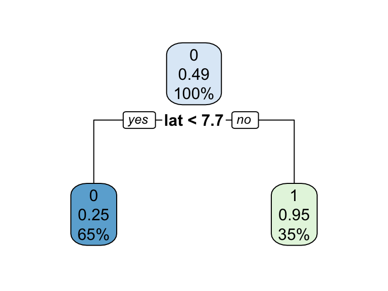

# plot tree 
par(mar = c(1, 1, 1, 1))
rpart.plot(mdl)

Figure 1: Decision tree illustrating the single split on feature x (left).

2.2 Partition, depth=default

# decision tree with defaults
mdl <- rpart(present ~ ., data = d_train)
mdl

n= 788 

node), split, n, loss, yval, (yprob)
      * denotes terminal node

  1) root 788 389 0 (0.50634518 0.49365482)  
    2) lat< 7.7401 512 128 0 (0.75000000 0.25000000)  
      4) WC_bio2>=10.25 247  22 0 (0.91093117 0.08906883) *
      5) WC_bio2< 10.25 265 106 0 (0.60000000 0.40000000)  
       10) WC_bio1>=26.15 87  10 0 (0.88505747 0.11494253) *
       11) WC_bio1< 26.15 178  82 1 (0.46067416 0.53932584)  
         22) lat>=0.617405 32   5 0 (0.84375000 0.15625000) *
         23) lat< 0.617405 146  55 1 (0.37671233 0.62328767)  
           46) lat< -2.529476 77  36 0 (0.53246753 0.46753247)  
             92) lat>=-16.94087 45   8 0 (0.82222222 0.17777778)  
              184) WC_bio2>=7.2 38   2 0 (0.94736842 0.05263158) *
              185) WC_bio2< 7.2 7   1 1 (0.14285714 0.85714286) *
             93) lat< -16.94087 32   4 1 (0.12500000 0.87500000) *
           47) lat>=-2.529476 69  14 1 (0.20289855 0.79710145)  
             94) lon>=-75.44386 33  12 1 (0.36363636 0.63636364)  
              188) WC_alt>=67 12   0 0 (1.00000000 0.00000000) *
              189) WC_alt< 67 21   0 1 (0.00000000 1.00000000) *
             95) lon< -75.44386 36   2 1 (0.05555556 0.94444444) *
    3) lat>=7.7401 276  15 1 (0.05434783 0.94565217) *

rpart.plot(mdl)

# plot complexity parameter
plotcp(mdl)

# rpart cross validation results
mdl$cptable

          CP nsplit rel error    xerror       xstd
1 0.63239075      0 1.0000000 1.1028278 0.03593877
2 0.03084833      1 0.3676093 0.3958869 0.02861490
3 0.01542416      6 0.2005141 0.2699229 0.02452406
4 0.01285347      8 0.1696658 0.2622108 0.02422420
5 0.01000000      9 0.1568123 0.2596401 0.02412272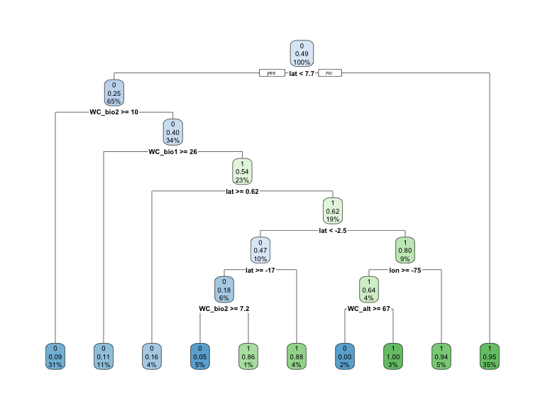

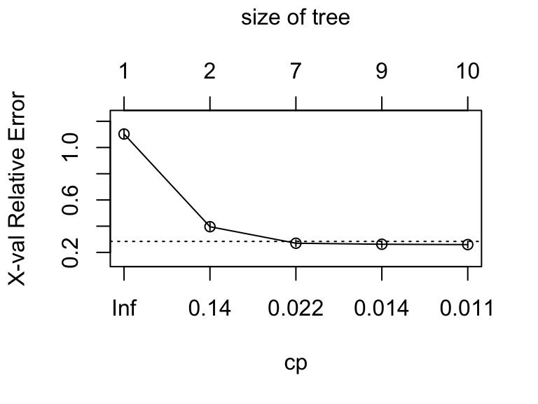
Figure 2: Decision tree $present$ classification.

2.3 Feature interpretation

# caret cross validation results
mdl_caret <- train(
  present ~ .,
  data       = d_train,
  method     = "rpart",
  trControl  = trainControl(method = "cv", number = 10),
  tuneLength = 20)

ggplot(mdl_caret)

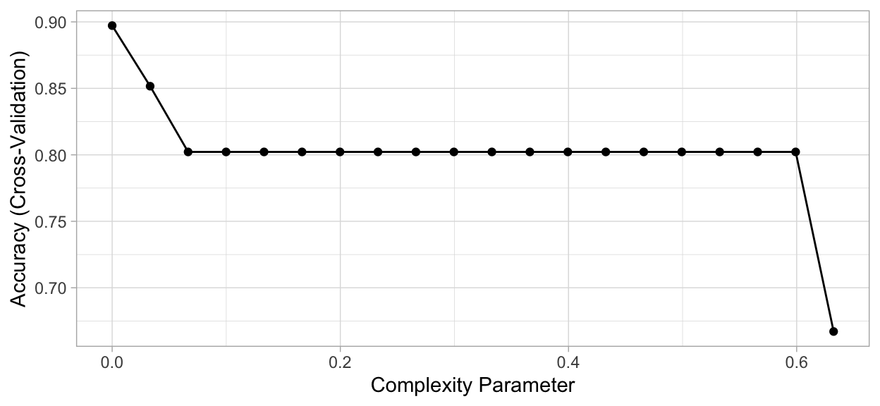
$Cross-validated accuracy rate for the 20 different $\alpha$ parameter values in our grid search. Lower $\alpha$ values (deeper trees) help to minimize errors.$

Figure 3: Cross-validated accuracy rate for the 20 different $\alpha$ parameter values in our grid search. Lower $\alpha$ values (deeper trees) help to minimize errors.

vip(mdl_caret, num_features = 40, bar = FALSE)

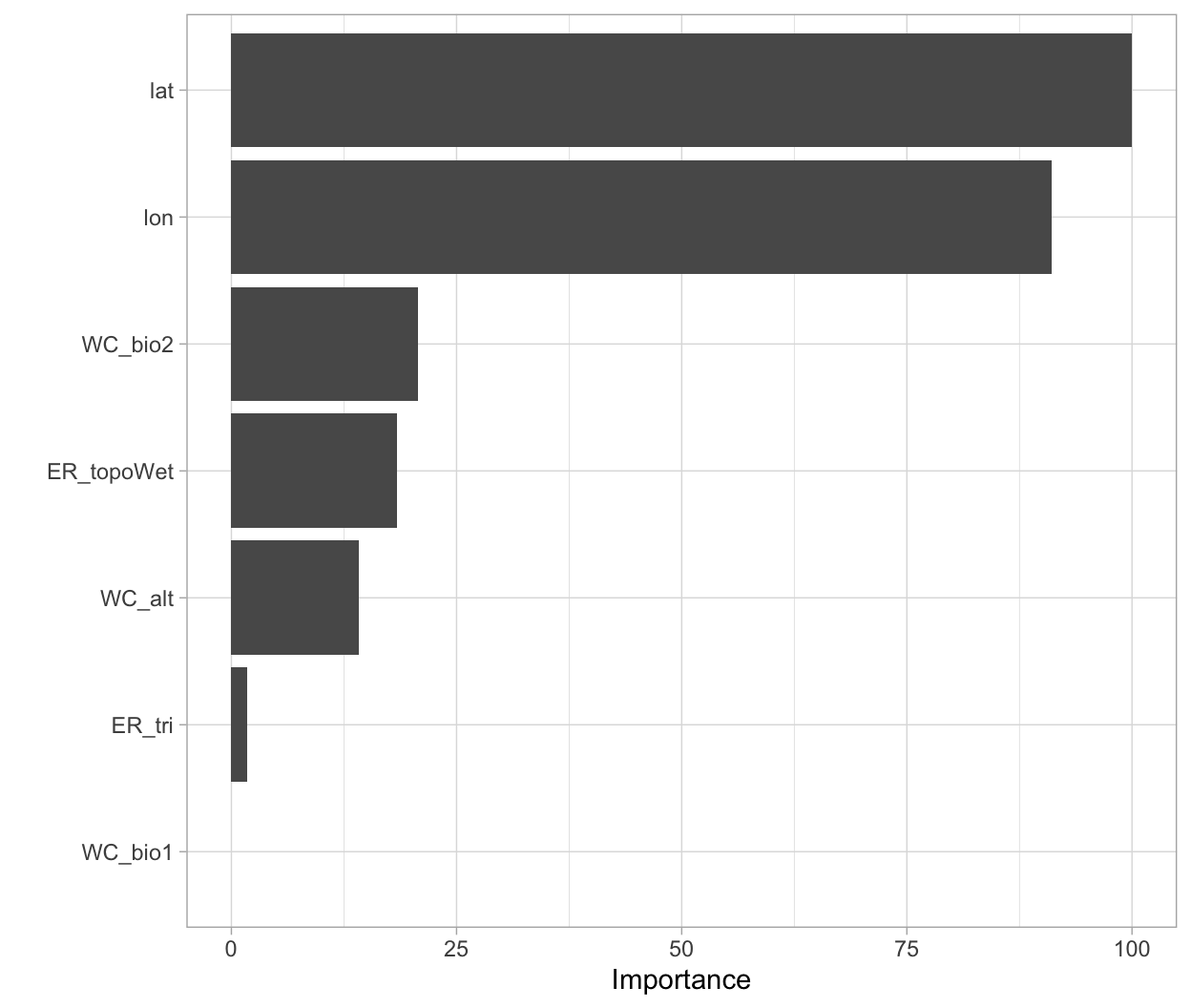
Figure 4: Variable importance based on the total reduction in MSE for the Ames Housing decision tree.

# Construct partial dependence plots
p1 <- partial(mdl_caret, pred.var = "lat") %>% autoplot()
p2 <- partial(mdl_caret, pred.var = "WC_bio2") %>% autoplot()
p3 <- partial(mdl_caret, pred.var = c("lat", "WC_bio2")) %>% 
  plotPartial(levelplot = FALSE, zlab = "yhat", drape = TRUE, 
              colorkey = TRUE, screen = list(z = -20, x = -60))

# Display plots side by side
gridExtra::grid.arrange(p1, p2, p3, ncol = 3)

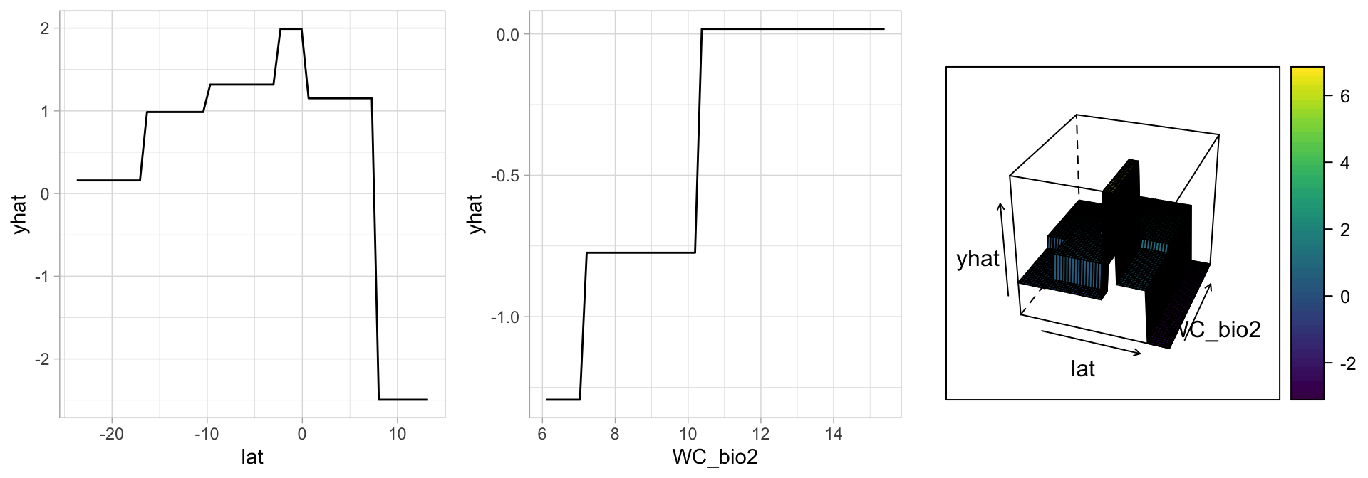
Figure 5: Partial dependence plots to understand the relationship between lat, WC_bio2 and present.

3 Random Forests

Reading: Boehmke & Greenwell (2020) Hands-On Machine Learning with R. Chapter 11 Random Forests

3.1 Fit

# number of features
n_features <- length(setdiff(names(d_train), "present"))

# fit a default random forest model
mdl_rf <- ranger(present ~ ., data = d_train)

# get out of the box RMSE
(default_rmse <- sqrt(mdl_rf$prediction.error))

[1] 0.2518964

3.2 Feature interpretation

# re-run model with impurity-based variable importance
mdl_impurity <- ranger(
  present ~ ., data = d_train,
  importance = "impurity")

# re-run model with permutation-based variable importance
mdl_permutation <- ranger(
  present ~ ., data = d_train,
  importance = "permutation")

p1 <- vip::vip(mdl_impurity, bar = FALSE)
p2 <- vip::vip(mdl_permutation, bar = FALSE)

gridExtra::grid.arrange(p1, p2, nrow = 1)

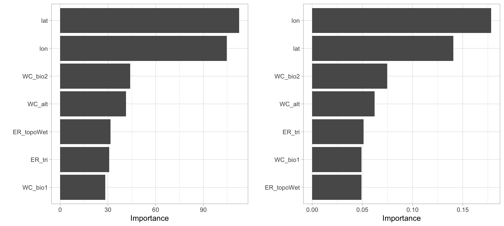
Figure 6: Most important variables based on impurity (left) and permutation (right).

Lab 1c. Species Distribution Modeling - Decision Trees