Learning Objectives
Now you’ll complete the modeling workflow with the steps to evaluate model performance and calibrate model parameters.
Figure 1: Full model workflow with calibrate and evaluate steps emphasized.
1 Setup
# global knitr chunk options
knitr::opts_chunk$set(
  warning = FALSE,
  message = FALSE)

# load packages
librarian::shelf(
  dismo, # species distribution modeling: maxent(), predict(), evaluate(),
  dplyr, ggplot2, GGally, here, maptools, readr,
  raster, readr, rsample, sf,
  usdm)  # uncertainty analysis for species distribution models: vifcor()
select = dplyr::select

# options
set.seed(42)
options(
  scipen = 999,
  readr.show_col_types = F)
ggplot2::theme_set(ggplot2::theme_light())

# paths
dir_data      <- here("data/sdm")
pts_geo       <- file.path(dir_data, "pts.geojson")
env_stack_grd <- file.path(dir_data, "env_stack.grd")
mdl_maxv_rds  <- file.path(dir_data, "mdl_maxent_vif.rds")

# read points of observation: presence (1) and absence (0)
pts <- read_sf(pts_geo)

# read raster stack of environment
env_stack <- raster::stack(env_stack_grd)
1.1 Split observations into training and testing
# create training set with 80% of full data
pts_split  <- rsample::initial_split(
  pts, prop = 0.8, strata = "present")
pts_train  <- rsample::training(pts_split)
pts_test   <- rsample::testing(pts_split)

pts_train_p <- pts_train %>%
  filter(present == 1) %>%
  as_Spatial()
pts_train_a <- pts_train %>%
  filter(present == 0) %>%
  as_Spatial()
2 Calibrate: Model Selection
# show pairs plot before multicollinearity reduction with vifcor()
pairs(env_stack)
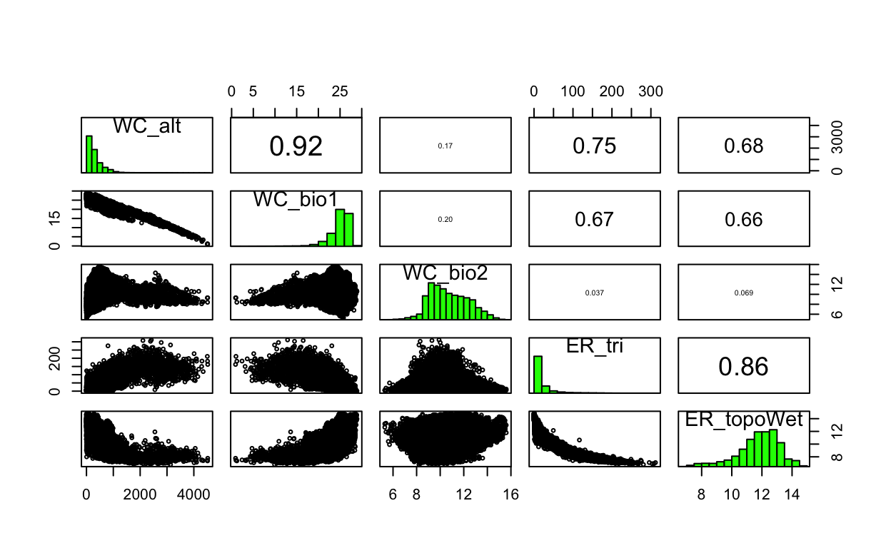
# calculate variance inflation factor per predictor, a metric of multicollinearity between variables
vif(env_stack)
   Variables      VIF
1     WC_alt 8.254995
2    WC_bio1 6.948011
3    WC_bio2 1.140249
4     ER_tri 5.066341
5 ER_topoWet 4.059576
# stepwise reduce predictors, based on a max correlation of 0.7 (max 1)
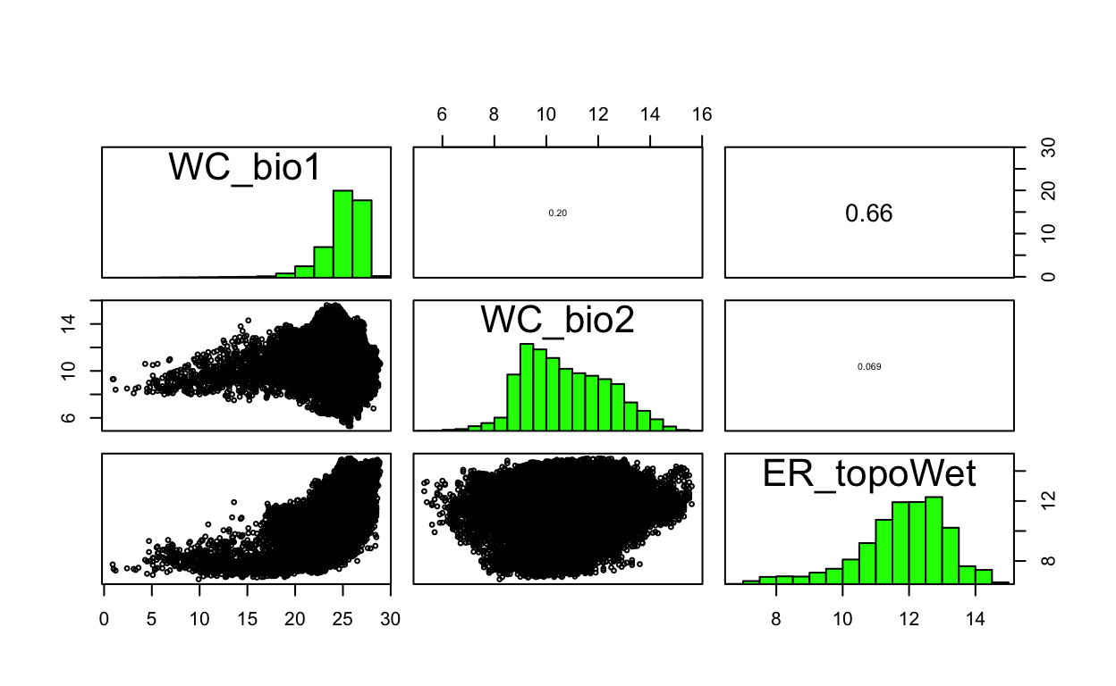
v <- vifcor(env_stack, th=0.7)
v
2 variables from the 5 input variables have collinearity problem:

WC_alt ER_tri

After excluding the collinear variables, the linear correlation coefficients ranges between:
min correlation ( ER_topoWet ~ WC_bio2 ):  -0.06974524
max correlation ( ER_topoWet ~ WC_bio1 ):  0.6474975

---------- VIFs of the remained variables --------
   Variables      VIF
1    WC_bio1 1.785410
2    WC_bio2 1.041940
3 ER_topoWet 1.730377
# reduce enviromental raster stack by
env_stack_v <- usdm::exclude(env_stack, v)
# show pairs plot after multicollinearity reduction with vifcor()
pairs(env_stack_v)
# fit a maximum entropy model
if (!file.exists(mdl_maxv_rds)){
mdl_maxv <- maxent(env_stack_v, sf::as_Spatial(pts_train))
readr::write_rds(mdl_maxv, mdl_maxv_rds)
}
mdl_maxv <- read_rds(mdl_maxv_rds)
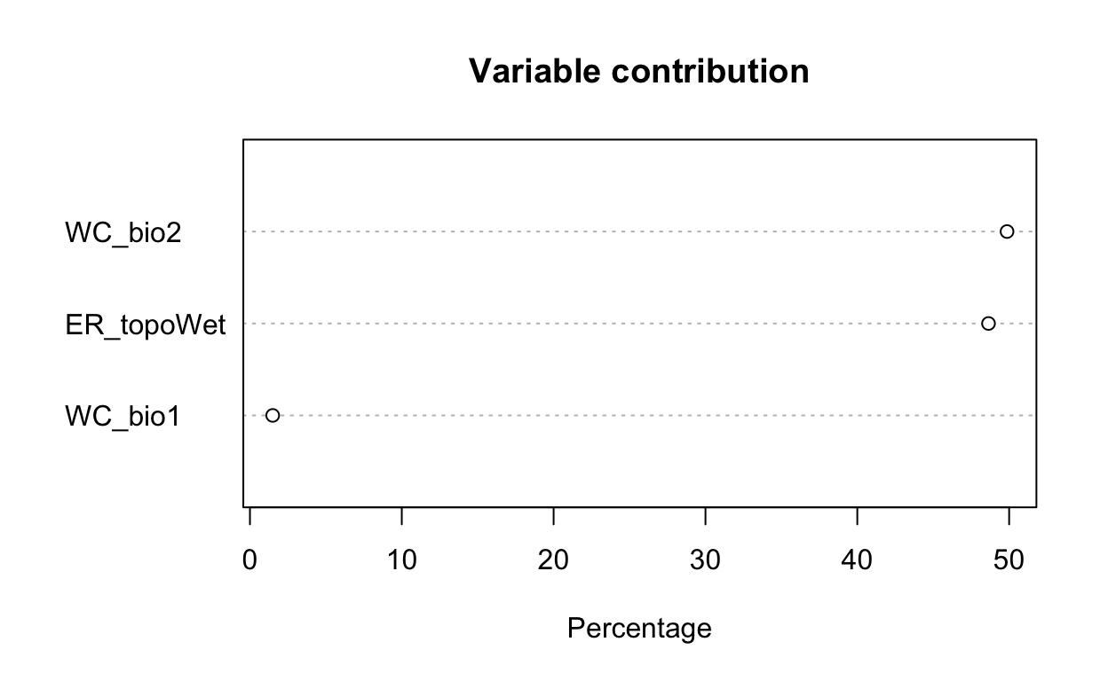
# plot variable contributions per predictor
plot(mdl_maxv)
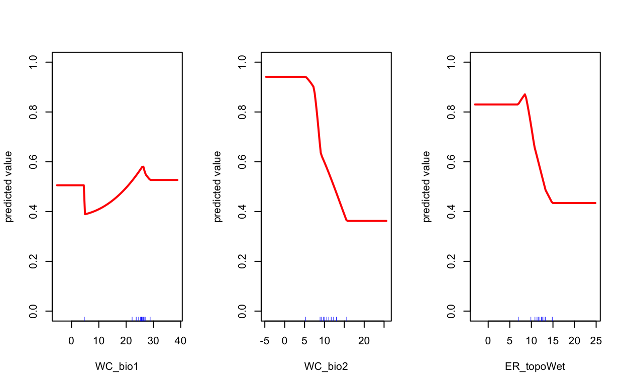
# plot term plots
response(mdl_maxv)
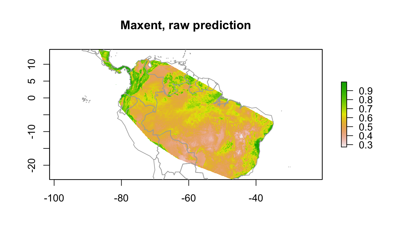
# predict
y_maxv <- predict(env_stack, mdl_maxv) #, ext=ext, progress='')

plot(y_maxv, main='Maxent, raw prediction')
data(wrld_simpl, package="maptools")
plot(wrld_simpl, add=TRUE, border='dark grey')
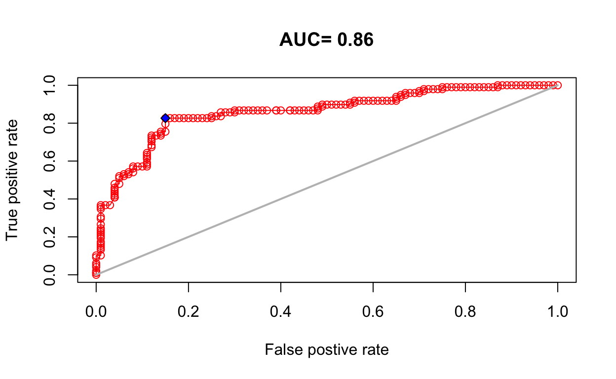
3 Evaluate: Model Performance
3.1 Area Under the Curve (AUC), Reciever Operater Characteristic (ROC) Curve and Confusion Matrix
pts_test_p <- pts_test %>%
  filter(present == 1) %>%
  as_Spatial()
pts_test_a <- pts_test %>%
  filter(present == 0) %>%
  as_Spatial()

y_maxv <- predict(mdl_maxv, env_stack)
#plot(y_maxv)

e <- dismo::evaluate(
  p     = pts_test_p,
  a     = pts_test_a,
  model = mdl_maxv,
  x     = env_stack)
e
class          : ModelEvaluation
n presences    : 98
n absences     : 100
AUC            : 0.8598469
cor            : 0.6240488
max TPR+TNR at : 0.6251154 plot(e, 'ROC')
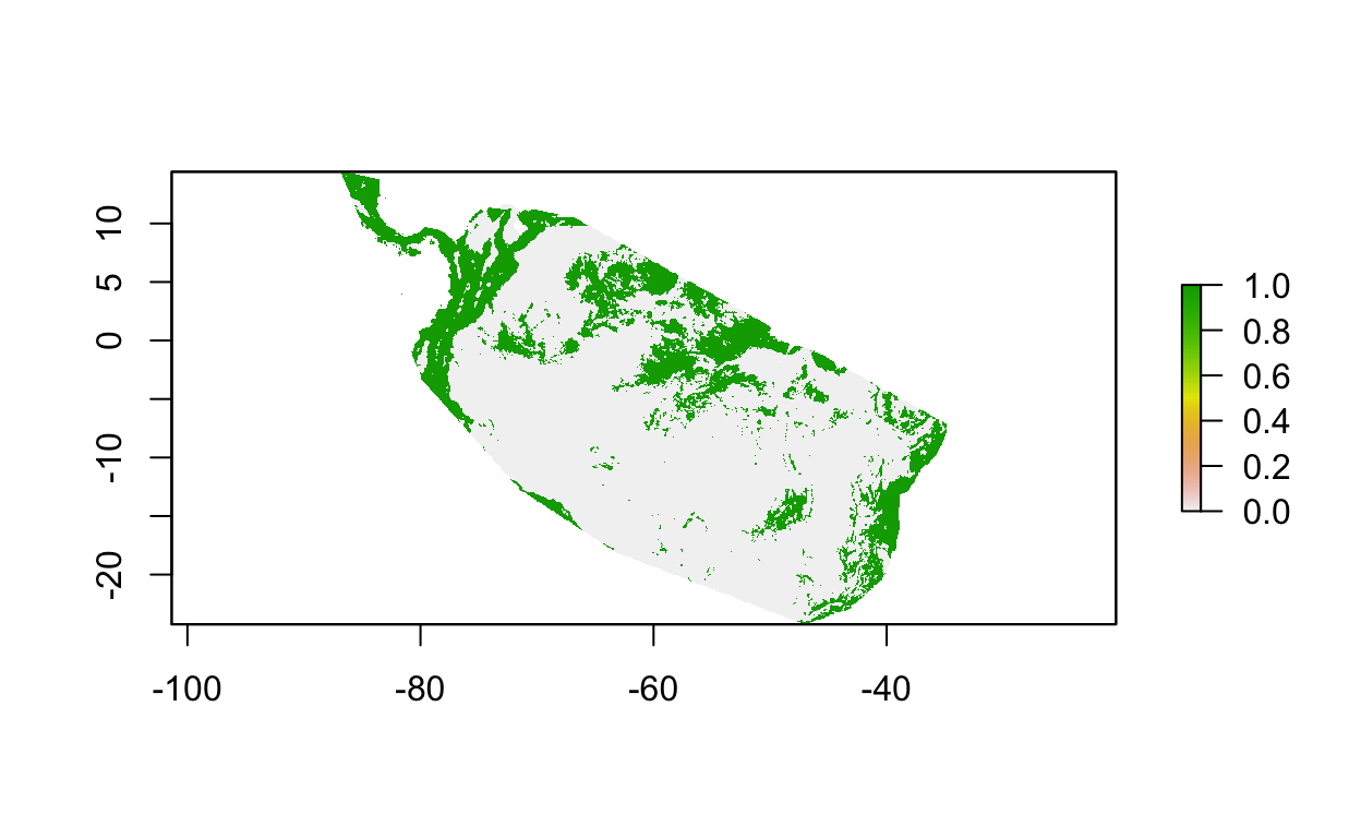
thr <- threshold(e)[['spec_sens']]
thr
[1] 0.6251154p_true <- na.omit(raster::extract(y_maxv, pts_test_p) >= thr)
a_true <- na.omit(raster::extract(y_maxv, pts_test_a) < thr)
# (t)rue/(f)alse (p)ositive/(n)egative rates
tpr <- sum(p_true)/length(p_true)
fnr <- sum(!p_true)/length(p_true)
fpr <- sum(!a_true)/length(a_true)
tnr <- sum(a_true)/length(a_true)
matrix(
c(tpr, fnr,
fpr, tnr),
nrow=2, dimnames = list(
c("present_obs", "absent_obs"),
c("present_pred", "absent_pred")))
            present_pred absent_pred
present_obs    0.8265306        0.15
absent_obs     0.1734694        0.85
# add point to ROC plot
points(fpr, tpr, pch=23, bg="blue")
plot(y_maxv > thr)
4 Lab1 Submission
To submit Lab 1, please submit the path on taylor.bren.ucsb.edu to your single consolidated Rmarkdown document (i.e. combined from separate parts) that you successfully knitted here:
The path should start /Users/ and end in .Rmd. Please be sure to have succesfully knitted to html, as in I should see the .html file there by the same name.
In your lab, please be sure to include:
| # | Lab | Item | Points |
|---|---|---|---|
| 1 | 1a.Explore | Name _Genus species_ used to search GBIF for observations. (0.5 pts) | 0.5 |
| 2 | 1a.Explore | Image of your species. I like to see wildlife. | 0.5 |
| 3 | 1a.Explore | Map of distribution of points | 0.5 |
| 4 | 1a.Explore | Question: How many observations total are in GBIF for your species? | 0.5 |
| 5 | 1a.Explore | Question: Did you have to perform any data cleaning steps? | 0.5 |
| 6 | 1a.Explore | Question: What environmental layers did you choose as predictors? Can you find any support for these in the literature? | 1 |
| 7 | 1a.Explore | Raster plot of environmental rasters clipped to species range | 0.5 |
| 8 | 1a.Explore | Map with pseudo-absence points | 0.5 |
| 9 | 1a.Explore | Term plots | 0.5 |
| 10 | 1b.Regress | Plot of ggpairs | 0.4 |
| 11 | 1b.Regress | Linear model output with range of values | 0.4 |
| 12 | 1b.Regress | Generalized Linear Model (GLM) output | 0.4 |
| 13 | 1b.Regress | GLM term plots | 0.3 |
| 14 | 1b.Regress | Generalized Additive Model (GAM) output | 0.3 |
| 15 | 1b.Regress | GAM term plots | 0.3 |
| 16 | 1b.Regress | Question: Which GAM environmental variables, and even range of values, seem to contribute most towards presence (above 0 response) versus absence (below 0 response)? | 1 |
| 17 | 1b.Regress | Maxent model output | 0.3 |
| 18 | 1b.Regress | Maxent variable contribution plot | 0.3 |
| 19 | 1b.Regress | Maxent term plots | 0.3 |
| 20 | 1b.Regress | Question: Which Maxent environmental variables, and even range of values, seem to contribute most towards presence (closer to 1 response) and how might this differ from the GAM results? | 1 |
| 21 | 1c.Trees | Tabular counts of 1 vs 0 before and after split | 0.4 |
| 22 | 1c.Trees | Rpart model output and plot, depth=1 | 0.4 |
| 23 | 1c.Trees | Rpart model output and plot, depth=default | 0.3 |
| 24 | 1c.Trees | Rpart complexity parameter plot | 0.3 |
| 25 | 1c.Trees | Question: Based on the complexity plot threshold, what size of tree is recommended? | 1 |
| 26 | 1c.Trees | Rpart variable importance plot | 0.3 |
| 27 | 1c.Trees | Question: what are the top 3 most important variables of your model? | 1 |
| 28 | 1c.Trees | RandomForest variable importance | 0.3 |
| 29 | 1c.Trees | Question: How might variable importance differ between rpart and RandomForest in your model outputs? | 1 |
| 30 | 1d.Evaluate | Plot of pairs from environmental stack | 0.3 |
| 31 | 1d.Evaluate | VIF per variable | 0.3 |
| 32 | 1d.Evaluate | Variables after VIF collinearity removal | 0.3 |
| 33 | 1d.Evaluate | Plof of pairs after VIF collinearity removal | 0.3 |
| 34 | 1d.Evaluate | Plot of variable contribution | 0.3 |
| 35 | 1d.Evaluate | Question: Which variables were removed due to multicollinearity and what is the rank of most to least important remaining variables in your model? | 1 |
| 36 | 1d.Evaluate | Maxent term plots | 0.4 |
| 37 | 1d.Evaluate | Map of Maxent prediction | 0.4 |
| 38 | 1d.Evaluate | ROC threshold value maximizing specificity and sensitivity | 0.4 |
| 39 | 1d.Evaluate | Confusion matrix with percentages | 0.5 |
| 40 | 1d.Evaluate | AUC plot | 0.4 |
| 41 | 1d.Evaluate | Map of binary habitat | 0.4 |