Example script demonstrating how to use the dismapr package for retrieving interpolated distance-weighted biomass data from NOAA’s DisMAP.
1. Indicators
Example 1: Get indicators data for American Lobster in Northeast US Spring
tbl_lobster_indicators <- dm_get_indicators(
  common_name = "American lobster",
  region      = "Northeast US",
  season      = "Spring")
tbl_lobster_indicators
#> # A tibble: 46 × 27
#>    objectid dataset_code region       season date_code species       common_name
#>       <int> <chr>        <chr>        <chr>  <chr>     <chr>         <chr>
#>  1     9866 NEUS_SPR     Northeast US Spring 20240701  Homarus amer… American l…
#>  2     9867 NEUS_SPR     Northeast US Spring 20240701  Homarus amer… American l…
#>  3     9868 NEUS_SPR     Northeast US Spring 20240701  Homarus amer… American l…
#>  4     9869 NEUS_SPR     Northeast US Spring 20240701  Homarus amer… American l…
#>  5     9870 NEUS_SPR     Northeast US Spring 20240701  Homarus amer… American l…
#>  6     9871 NEUS_SPR     Northeast US Spring 20240701  Homarus amer… American l…
#>  7     9872 NEUS_SPR     Northeast US Spring 20240701  Homarus amer… American l…
#>  8     9873 NEUS_SPR     Northeast US Spring 20240701  Homarus amer… American l…
#>  9     9874 NEUS_SPR     Northeast US Spring 20240701  Homarus amer… American l…
#> 10     9875 NEUS_SPR     Northeast US Spring 20240701  Homarus amer… American l…
#> # ℹ 36 more rows
#> # ℹ 20 more variables: core_species <chr>, year <int>,
#> #   distribution_project_name <chr>, distribution_project_code <chr>,
#> #   summary_product <chr>, center_of_gravity_latitude <dbl>,
#> #   minimum_latitude <dbl>, maximum_latitude <dbl>, offset_latitude <dbl>,
#> #   center_of_gravity_latitude_se <dbl>, center_of_gravity_longitude <dbl>,
#> #   minimum_longitude <dbl>, maximum_longitude <dbl>, offset_longitude <dbl>, …

# plot center of gravity changes over time
dm_plot_indicators(
  tbl_lobster_indicators,
  title = "American Lobster Center of Gravity")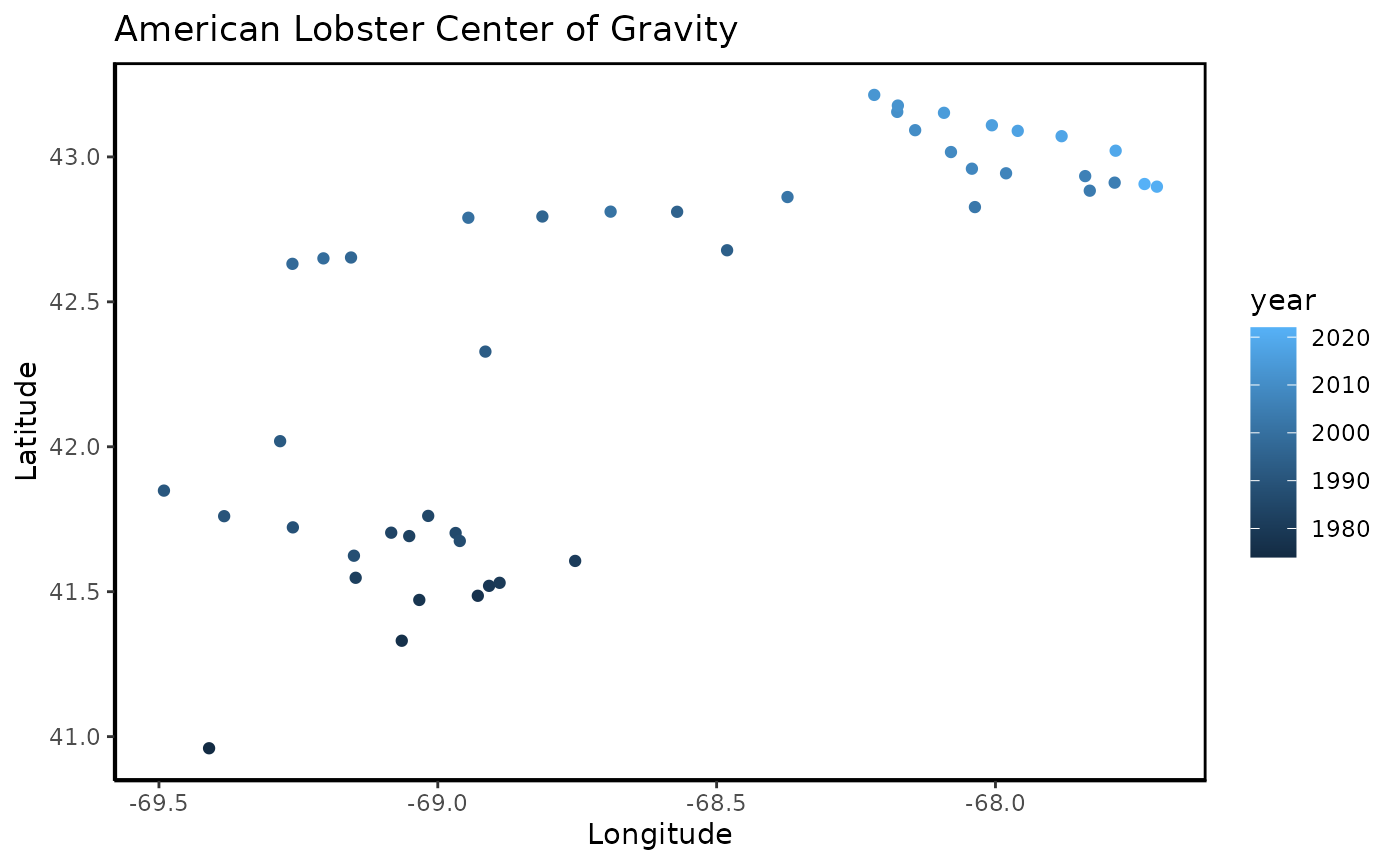
2. Rasters
Example 2: Download interpolated biomass rasters for Summer Flounder in NEUS Spring
# show table of dataset_codes for available regions and seasons
dm_datasets |>
  sf::st_drop_geometry() |>
  DT::datatable()
# show map of dataset_codes
dm_plot_datasets(dm_datasets)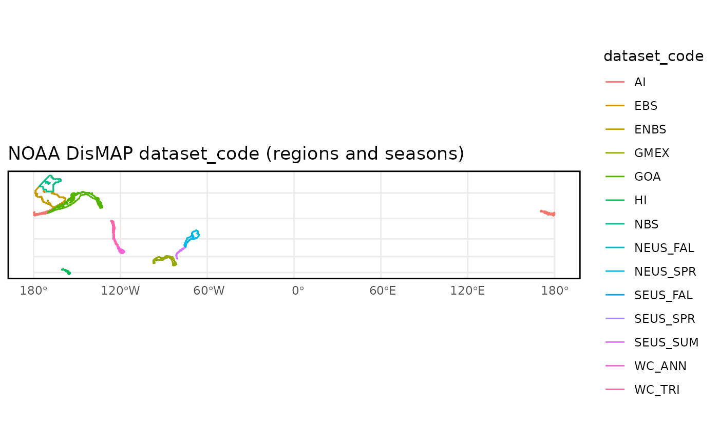
# pick the Northeast US Spring dataset
dataset_code <- "NEUS_SPR"

# show list of available region_seasons (where season may be optional)
dm_get_dataset_layers(dataset_code)
#>  [1] "Alosa aestivalis"                "Alosa pseudoharengus"
#>  [3] "Alosa sapidissima"               "Amblyraja radiata"
#>  [5] "Anarhichas lupus"                "Cancer irroratus"
#>  [7] "Centropristis striata"           "Chaceon quinquedens"
#>  [9] "Clupea harengus"                 "Core Species Richness"
#> [11] "Dipturus laevis"                 "Doryteuthis pealeii"
#> [13] "Gadus morhua"                    "Glyptocephalus cynoglossus"
#> [15] "Hemitripterus americanus"        "Hippoglossina oblonga"
#> [17] "Hippoglossoides platessoides"    "Hippoglossus hippoglossus"
#> [19] "Homarus americanus"              "Illex illecebrosus"
#> [21] "Leucoraja erinaceus"             "Leucoraja garmani"
#> [23] "Leucoraja ocellata"              "Limulus polyphemus"
#> [25] "Lophius americanus"              "Malacoraja senta"
#> [27] "Melanogrammus aeglefinus"        "Merluccius albidus"
#> [29] "Merluccius bilinearis"           "Micropogonias undulatus"
#> [31] "Myoxocephalus octodecemspinosus" "Myzopsetta ferruginea"
#> [33] "Paralichthys dentatus"           "Peprilus triacanthus"
#> [35] "Phycis chesteri"                 "Placopecten magellanicus"
#> [37] "Pollachius virens"               "Prionotus carolinus"
#> [39] "Pseudopleuronectes americanus"   "Rostroraja eglanteria"
#> [41] "Scomber scombrus"                "Scophthalmus aquosus"
#> [43] "Sebastes fasciatus"              "Species Richness"
#> [45] "Squalus acanthias"               "Urophycis chuss"
#> [47] "Urophycis regia"                 "Urophycis tenuis"
#> [49] "Zoarces americanus"

# pick the layer (i.e., species): summer flounder (Paralichthys dentatus)
layer     <- "Paralichthys dentatus"
sp_common <- "SummerFlounder"

# show list of available years
dm_get_dataset_layer_years(dataset_code, layer)
#>  [1] 1974 1976 1977 1978 1979 1980 1981 1982 1983 1984 1985 1986 1987 1988 1989
#> [16] 1990 1991 1992 1993 1994 1995 1996 1997 1998 1999 2000 2001 2002 2003 2004
#> [31] 2005 2006 2007 2008 2009 2010 2011 2012 2013 2015 2016 2017 2018 2019 2021
#> [46] 2022

# pick a set of years
years <- 2015:2019

# create directory for downloads
output_dir <- here::here("inst/test")
dir.create(output_dir, showWarnings = F, recursive = T)

# download each raster
for (yr in years) { # yr = years[1]
  tif <- glue::glue("{output_dir}/{dataset_code}_IDW_{sp_common}_{yr}.tif")

  r <- dm_get_raster(
    dataset_code,
    layer,
    yr,
    tif)
}

yr <- 2015
r <- terra::rast(glue::glue("{output_dir}/{dataset_code}_IDW_{sp_common}_{yr}.tif"))
r
#> class       : SpatRaster
#> dimensions  : 400, 400, 1  (nrow, ncol, nlyr)
#> resolution  : 2660, 2660  (x, y)
#> extent      : 321350, 1385350, 3888846, 4952846  (xmin, xmax, ymin, ymax)
#> coord. ref. : NAD83(2011) / UTM zone 18N (EPSG:6347)
#> source      : NEUS_SPR_IDW_SummerFlounder_2015.tif
#> name        :   wtcpue
#> min value   : 0.000000
#> max value   : 3.629863
Plot raster
# interactive plot
dm_plot_raster(
  r,
  interactive = TRUE,
  main = glue::glue("{dataset_code} {sp_common}, {yr}"))
# static plot
dm_plot_raster(
  r,
  interactive = FALSE,
  title = glue::glue("{dataset_code} {sp_common}, {yr}"))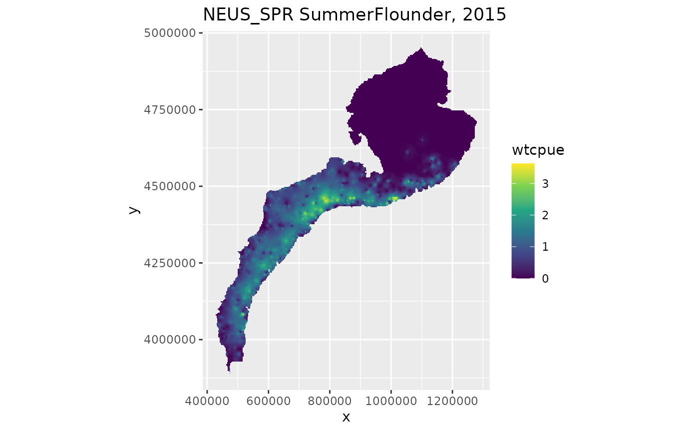
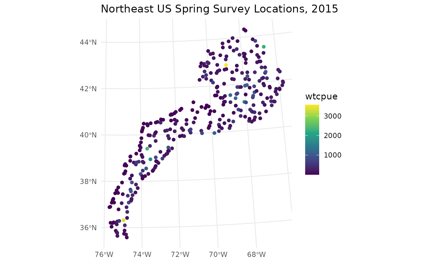
3. Surveys
dataset_code <- "NEUS_SPR"
year <- 2015

pts_yr <- dm_get_survey_locations(dataset_code, where = glue::glue("Year = {year}"))
# show a sample of first 100 rows
head(pts_yr, 100) |>
  DT::datatable()
# summarize by biomass
pts_yr_sum <- pts_yr |>
  dplyr::group_by(Longitude, Latitude) |>
  dplyr::summarize(
    wtcpue = sum(WTCPUE), .groups = "drop")

# interactive plot
dm_plot_survey_locations(
  pts_yr_sum,
  interactive = TRUE,
  title = glue::glue("Northeast US Spring Survey Locations, {year}"))
# static plot
dm_plot_survey_locations(
  pts_yr_sum,
  interactive = FALSE,
  title = glue::glue("Northeast US Spring Survey Locations, {year}"))