Lesson 2 Interactive Maps
2.1 Overview
Questions
- How do you generate interactive plots of spatial data to enable pan, zoom and hover/click for more detail?
Objectives
Learn variety of methods for producing interactive spatial output using libraries:
plotly: makes any ggplot2 object interactivemapview: quick view of any spatial objectleaflet: full control over interactive map
2.2 Things You’ll Need to Complete this Tutorial
R Skill Level: Intermediate - you’ve got basics of R down.
We will continue to use the sf and raster packages and introduce the plotly, mapview, and leaflet packages in this tutorial.
# load packages
library(tidyverse)  # loads dplyr, tidyr, ggplot2 packages
library(sf)         # simple features package - vector
library(raster)     # raster
library(plotly)     # makes ggplot objects interactive
library(mapview)    # quick interactive viewing of spatial objects
library(leaflet)    # interactive maps

# set working directory to data folder
# setwd("pathToDirHere")
2.3 States: ggplot2
Recreate the ggplot object from Lesson 1 and save into a variable for subsequent use with the plotly package.
# read in states
states <- read_sf("data/NEON-DS-Site-Layout-Files/US-Boundary-Layers/US-State-Boundaries-Census-2014.shp") %>%
  st_zm() %>%
  mutate(
    water_km2 = (AWATER / (1000*1000)) %>% round(2))

# plot, ggplot
g = ggplot(states) +
  geom_sf(aes(fill = water_km2)) +
  scale_fill_distiller("water_km2", palette = "Spectral") +
  ggtitle("Water (km2) by State")
g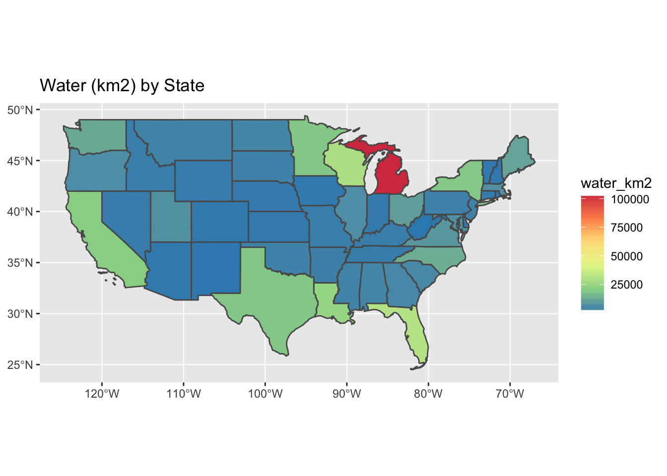
2.4 States: plotly
The plotly::ggplotly() function outputs a ggplot into an interactive window capable of pan, zoom and identify.
library(plotly)

ggplotly(g)
2.5 States: mapview
The mapview::mapview() function can work for a quick view of the data, providing choropleths, background maps and attribute popups. Performance varies on the object and customization can be tricky.
library(mapview)

# simple view with popups
mapview(states)
# coloring and layering
mapview(states, zcol='water_km2', burst='STUSPS')2.6 States: leaflet
The leaflet package offers a robust set of functions for viewing vector and raster data, although requires more explicit functions.
library(leaflet)

leaflet(states) %>%
  addTiles() %>%
  addPolygons()
2.6.1 Choropleth
Drawing from the documentation from Leaflet for R - Choropleths, we can construct a pretty choropleth.
pal <- colorBin("Blues", domain = states$water_km2, bins = 7)


leaflet(states) %>%
  addProviderTiles("Stamen.TonerLite") %>%
  addPolygons(
    # fill
    fillColor   = ~pal(water_km2),
    fillOpacity = 0.7,
    # line
    dashArray   = "3",
    weight      = 2,
    color       = "white",
    opacity     = 1,
    # interaction
    highlight = highlightOptions(
      weight = 5,
      color = "#666",
      dashArray = "",
      fillOpacity = 0.7,
      bringToFront = TRUE))
2.6.2 Popups and Legend
Adding a legend and popups requires a bit more work, but achieves a very aesthetically and functionally pleasing visualization.
library(htmltools)
library(scales)

labels <- sprintf(
  "<strong>%s</strong><br/> water: %s km<sup>2</sup>",
  states$NAME, comma(states$water_km2)) %>%
  lapply(HTML)

leaflet(states) %>%
  addProviderTiles("Stamen.TonerLite") %>%
  addPolygons(
    # fill
    fillColor   = ~pal(water_km2),
    fillOpacity = 0.7,
    # line
    dashArray   = "3",
    weight      = 2,
    color       = "white",
    opacity     = 1,
    # interaction
    highlight = highlightOptions(
      weight = 5,
      color = "#666",
      dashArray = "",
      fillOpacity = 0.7,
      bringToFront = TRUE),
  label = labels,
  labelOptions = labelOptions(
    style = list("font-weight" = "normal", padding = "3px 8px"),
    textsize = "15px",
    direction = "auto")) %>%
  addLegend(
    pal = pal, values = ~water_km2, opacity = 0.7, title = HTML("Water (km<sup>2</sup>)"),
    position = "bottomright")
2.7 Challenge: leaflet for regions
Use Lesson 1 final output to create a regional choropleth with legend and popups for percent water by region.
2.7.1 Answers
regions = states %>%
  group_by(region) %>%
  summarize(
    water = sum(AWATER),
    land  = sum(ALAND)) %>%
  mutate(
    pct_water = (water / land * 100) %>% round(2))

pal <- colorBin("Spectral", domain = regions$pct_water, bins = 5)

labels <- sprintf(
  "<strong>%s</strong><br/>water: %s%%",
  regions$region, comma(regions$pct_water)) %>%
  lapply(HTML)

leaflet(regions) %>%
  addProviderTiles("Stamen.TonerLite") %>%
  addPolygons(
    # fill
    fillColor   = ~pal(pct_water),
    fillOpacity = 0.7,
    # line
    dashArray   = "3",
    weight      = 2,
    color       = "white",
    opacity     = 1,
    # interaction
    highlight = highlightOptions(
      weight = 5,
      color = "#666",
      dashArray = "",
      fillOpacity = 0.7,
      bringToFront = TRUE),
  label = labels,
  labelOptions = labelOptions(
    style = list("font-weight" = "normal", padding = "3px 8px"),
    textsize = "15px",
    direction = "auto")) %>%
  addLegend(
    pal = pal, values = ~pct_water, opacity = 0.7, title = "water %",
    position = "bottomright")
2.8 Raster: leaflet
TODO: show raster overlay using NEON raster dataset example
2.9 Key Points
- Interactive maps provide more detail for visual investigation, including use of background maps, but is only relevant in a web context.
- Several packages exist for providing interactive views of data.
- The
plotly::ggplotly()function works quickly if you already have a ggplot object, which is best for static output. - The
mapview::mapview()function can work for a quick view of the data, providing choropleths, background maps and attribute popups. Performance varies on the object and customization can be tricky. - The
leafletpackage provides a highly customizable set of functions for rendering of interactive choropleths with background maps, legends, etc.